# - - - - - - - - - - - - - - - - - - - - - - - - - - - - - - - - - - - - - - - #
# A Simple Skript for planecrash data from:
# http://www.planecrashinfo.com/database.htm
# The aviation accident database includes:
# All civil and commercial aviation accidents of scheduled and non-scheduled
# passenger airliners worldwide, which resulted in a fatality
# (including all U.S. Part 121 and Part 135 fatal accidents)
# All cargo, positioning, ferry and test flight fatal accidents.
# All military transport accidents with 10 or more fatalities.
# All commercial and military helicopter accidents with greater than
# 10 fatalities.
# All civil and military airship accidents involving fatalities.
# Aviation accidents involving the death of famous people.
# Aviation accidents or incidents of noteworthy interest.
# Database Format
# Date: Date of accident, in the format - January 01, 2001
# Time: Local time, in 24 hr. format unless otherwise specified
# Airline/Op: Airline or operator of the aircraft
# Flight #: Flight number assigned by the aircraft operator
# Route: Complete or partial route flown prior to the accident
# AC Type: Aircraft type
# Reg: ICAO registration of the aircraft
# cn / ln: Construction or serial number / Line or fuselage number
# Aboard: Total aboard (passengers / crew)
# Fatalities: Total fatalities aboard (passengers / crew)
# Ground: Total killed on the ground
# Summary: Brief description of the accident and cause if known
# to be done: histograms, t test?, types of chrashes,
# country filter?, region filter, plane filter
# text analysis,
# - - - - - - - - - - - - - - - - - - - - - - - - - - - - - - - - - - - - - - - #
# packages
library("XML")
library("quantmod")
# - - - - - - - - - - - - - - - - - - - - - - - - - - - - - - - - - - - - - - - #
#
rm(list = ls(all = TRUE))
getwd()
#system("ls")
setwd("~/ownCloud/STA_Statistics/PlaneCrashData")
# - - - - - - - - - - - - - - - - - - - - - - - - - - - - - - - - - - - - - - - #
# get the available years
url <- "http://www.planecrashinfo.com/database.htm"
tables <- readHTMLTable(url,header=FALSE)
years <- NULL
for(i in 1:length(tables[[2]][,1])){
for(e in 2:length(tables[[2]][1,])){
years<-c(years,levels(tables[[2]][i,e])[i])
}
}
years
years<-na.omit(as.numeric(years))
years
# - - - - - - - - - - - - - - - - - - - - - - - - - - - - - - - - - - - - - - - #
# get all data tables
table.crash.all <- list()
for(i in 1:length(years)){
url2 <- paste("http://www.planecrashinfo.com/",
years[i],"/",years[i],".htm",sep="")
assign(paste("table.crash.",years[i],sep=""),readHTMLTable(url2))
table.crash.all[[i]] <- get(paste("table.crash.",years[i],sep=""))
print(paste("Year",years[i],"downloaded"))
}
#table.crash.all
length(table.crash.all)
save(table.crash.all,file="planecrashdata_list.RData")
for(i in 1:length(years)){
data<-table.crash.all[[i]]
save(data,file=paste("planecrashdata_",years[i],".RData",sep=""))
}
for(i in 1:length(years)){
data<-table.crash.all[[i]]
write.csv(data,file=paste("planecrashdata_",years[i],".csv",sep=""))
}
# - - - - - - - - - - - - - - - - - - - - - - - - - - - - - - - - - - - - - - - #
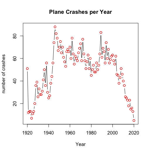
# Plane Crashes per Year
years.crashes <- data.frame()
for(i in 1:length(years)){
years.crashes[i,1] <- years[i]
years.crashes[i,2] <- length(as.data.frame(table.crash.all[[i]])[,1])
}
years.crashes
rownames(years.crashes)<-years.crashes[,1]
par(mfrow=c(1,1))
plot(years.crashes,type="b",main="Plane Crashes per Year",
xlab="Year",ylab="number of crashes")
points(years.crashes,col="red")
par(mfrow=c(1,1))
setwd("/Users/impac/ownCloud/STA_Statistics/PlaneCrashData/plots")
jpeg(file="Plane Crashes per Year-points.jpeg", width = 1080,
height = 1080, pointsize = 12, quality = 75)
plot(years.crashes,type="b",main="Plane Crashes per Year",
xlab="Year",ylab="number of crashes")
points(years.crashes,col="red")
dev.off()
jpeg(file="Plane Crashes per Year-bars.jpeg", width = 1080,
height = 1080, pointsize = 12, quality = 75)
plot(years.crashes,type="h",main="Plane Crashes per Year",
xlab="Year",ylab="number of crashes")
points(years.crashes,col="red")
dev.off()
jpeg(file="Plane Crashes per Year-steps.jpeg", width = 1080,
height = 1080, pointsize = 12, quality = 75)
plot(years.crashes,type="s",main="Plane Crashes per Year",
xlab="Year",ylab="number of crashes")
points(years.crashes,col="red")
dev.off()
par(mfrow=c(2,2))
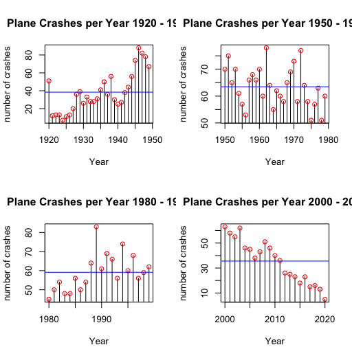
plot(years.crashes[1:30,],type="h",main=paste("Plane Crashes per Year",
years.crashes[1,1],"-",years.crashes[30,1]),xlab="Year",
ylab="number of crashes")
points(years.crashes[1:30,],col="red")
abline(h=mean(years.crashes[1:30,2]),col="blue")
plot(years.crashes[31:60,],type="h",main=paste("Plane Crashes per Year",years.crashes[31,1],"-",years.crashes[60,1]),xlab="Year",ylab="number of crashes")
points(years.crashes[31:60,],col="red")
abline(h=mean(years.crashes[31:60,2]),col="blue")
plot(years.crashes[61:80,],type="h",main=paste("Plane Crashes per Year",years.crashes[61,1],"-",years.crashes[80,1]),xlab="Year",ylab="number of crashes")
points(years.crashes[61:80,],col="red")
abline(h=mean(years.crashes[61:80,2]),col="blue")
plot(years.crashes[81:length(years.crashes[,1]),],type="h",main=paste("Plane Crashes per Year",years.crashes[81,1],"-",years.crashes[length(years.crashes[,1]),1]),xlab="Year",ylab="number of crashes")
points(years.crashes[81:length(years.crashes[,1]),],col="red")
abline(h=mean(years.crashes[81:length(years.crashes[,1]),2]),col="blue")
#jpeg(file="Plane Crashes per Year.jpeg", width = 1080, height = 1080, pointsize = 12, quality = 75)
#par(mfrow=c(2,2))
#plot(years.crashes[1:30,],type="h",main=paste("Plane Crashes per Year",years.crashes[1,1],"-",years.crashes[30,1]),xlab="Year",ylab="number of crashes")
#points(years.crashes[1:30,],col="red")
#abline(h=mean(years.crashes[1:30,2]),col="blue")
#plot(years.crashes[31:60,],type="h",main=paste("Plane Crashes per Year",years.crashes[31,1],"-",years.crashes[60,1]),xlab="Year",ylab="number of crashes")
#points(years.crashes[31:60,],col="red")
#abline(h=mean(years.crashes[31:60,2]),col="blue")
#plot(years.crashes[61:80,],type="h",main=paste("Plane Crashes per Year",years.crashes[61,1],"-",years.crashes[80,1]),xlab="Year",ylab="number of crashes")
#points(years.crashes[61:80,],col="red")
#abline(h=mean(years.crashes[61:80,2]),col="blue")
#plot(years.crashes[81:length(years.crashes[,1]),],type="h",main=paste("Plane Crashes per Year",years.crashes[81,1],"-",years.crashes[length(years.crashes[,1]),1]),xlab="Year",ylab="number of crashes")
#points(years.crashes[81:length(years.crashes[,1]),],col="red")
#abline(h=mean(years.crashes[81:length(years.crashes[,1]),2]),col="blue")
#dev.off()
# - - - - - - - - - - - - - - - - - - - - - - - - - - - - - - - - - - - - - - - #
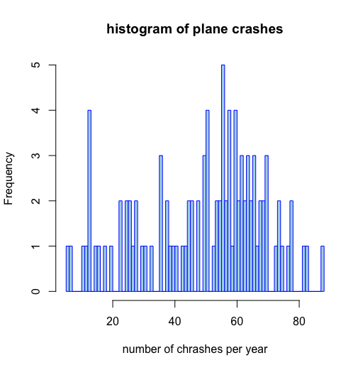
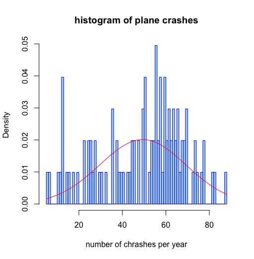
# Histograms of the number of crashes
par(mfrow=c(1,1))
hist(years.crashes[,2], nclass=length(years.crashes[,2]),
freq=TRUE, main='histogram of plane crashes',
xlab="number of chrashes per year", col = "lightblue", border = "blue")
hist(years.crashes[,2], nclass=length(years.crashes[,2]), freq=FALSE,
main='histogram of plane crashes',xlab="number of chrashes per year",
col = "lightblue", border = "blue")
curve(dnorm(x, mean=mean(years.crashes[,2]),sd=sd(years.crashes[,2])),
add=TRUE, col="red")
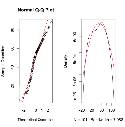
par(mfrow=c(1,2))
qqnorm(years.crashes[,2])
qqline(years.crashes[,2], col = 2)
plot(density(years.crashes[,2]),log='y', main='')
curve(dnorm(x, mean=mean(years.crashes[,2]),
sd=sd(years.crashes[,2])), log="y", add=TRUE, col="red")
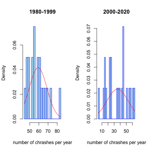
# different periods
par(mfrow=c(1,2))
# 1980-1999
#hist(years.crashes[61:80,2], nclass=20, freq=TRUE,
# main='',xlab="number of chrashes per year", col = "lightblue",
# border = "blue")
hist(years.crashes[61:80,2], nclass=20, freq=FALSE, main='1980-1999',xlab="number of chrashes per year", col = "lightblue", border = "blue")
curve(dnorm(x, mean=mean(years.crashes[61:80,2]),sd=sd(years.crashes[61:80,2])), add=TRUE, col="red")
# 2000-2020
#hist(years.crashes[81:length(years.crashes[,1]),2], nclass=length(years.crashes[81:length(years.crashes[,1]),2]), freq=TRUE, main='',xlab="number of chrashes per year", col = "lightblue", border = "blue")
hist(years.crashes[81:length(years.crashes[,1]),2], nclass=length(years.crashes[81:length(years.crashes[,1]),2]), freq=FALSE, main='2000-2020',xlab="number of chrashes per year", col = "lightblue", border = "blue")
curve(dnorm(x,mean=mean(years.crashes[81:length(years.crashes[,1]),2]),sd=sd(years.crashes[81:length(years.crashes[,1]),2])), add=TRUE, col="red")
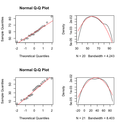
par(mfrow=c(2,2))
qqnorm(years.crashes[61:80,2])
qqline(years.crashes[61:80,2], col = 2)
plot(density(years.crashes[61:80,2]),log='y', main='')
curve(dnorm(x, mean=mean(years.crashes[61:80,2]),sd=sd(years.crashes[61:80,2])), log="y", add=TRUE, col="red")
qqnorm(years.crashes[81:length(years.crashes[,1]),2])
qqline(years.crashes[81:length(years.crashes[,1]),2], col = 2)
plot(density(years.crashes[81:length(years.crashes[,1]),2]),log='y', main='')
curve(dnorm(x, mean=mean(years.crashes[81:length(years.crashes[,1]),2]),sd=sd(years.crashes[81:length(years.crashes[,1]),2])), log="y", add=TRUE, col="red")
# - - - - - - - - - - - - - - - - - - - - - - - - - - - - - - - - - - - - - - - #
# boxplots
par(mfrow=c(1,1))
boxplot(years.crashes[,2], main="number of plain crashes per year 1920 - 2020", xlab="", ylab="plain crashes per year")
boxplot(years.crashes[,2], notch=TRUE, col=(c("gold","darkgreen")), main="number of plain crashes per year 1920 - 2020", ylab="plain crashes per year")
years.crashes[1:30,3]<-rep("1920-1949",30)
years.crashes[31:60,3]<-rep("1950-1979",30)278750
years.crashes[61:80,3]<-rep("1980-1999",20)
years.crashes[81:length(years.crashes[,1]),3]<-rep("2000-2020",21)
colnames(years.crashes)<-c("year","ncrashes","cat")
boxplot(ncrashes~cat, data=years.crashes, notch=TRUE, col=(c("green","blue","blue","green")), main="number of plain crashes per year - groups", xlab="")
# start from here
# - - - - - - - - - - - - - - - - - - - - - - - - - - - - - - - - - - - - - - - #
# - - - - - - - - - - - - - - - - - - - - - - - - - - - - - - - - - - - - - - - #
# t test
# independent 2-group t-test t.test(y~x) # where y is numeric and x is a binary factor
# independent 2-group t-test t.test(y1,y2) # where y1 and y2 are numeric
# paired t-test t.test(y1,y2,paired=TRUE) # where y1 & y2 are numeric
# one sample t-test t.test(y,mu=3) # Ho: mu=3
t.test(years.crashes[61:80,2],years.crashes[81:length(years.crashes[,1]),2])
# Welch Two Sample t-test
#
# data: years.crashes[61:80, 2] and years.crashes[81:length(years.crashes[, 1]), 2]
# t = 5.4142, df = 31.453, p-value = 6.268e-06
# alternative hypothesis: true difference in means is not equal to 0
# 95 percent confidence interval:
# 14.70178 32.45536
# sample estimates:
# mean of x mean of y
# 59.15000 35.57143
# - - - - - - - - - - - - - - - - - - - - - - - - - - - - - - - - - - - - - - - #
# rate of difference
par(mfrow=c(3,1))
rate<-na.omit(ROC(years.crashes[,2]))
plot(rate,type="l")
plot(cumsum(rate),type="l")
hist(rate, nclass=20)
rate<-na.omit(ROC(years.crashes[61:80,2]))
plot(rate,type="l")
plot(cumsum(rate),type="l")
hist(rate, nclass=20)
rate<-na.omit(ROC(years.crashes[81:length(years.crashes[,1]),2]))
plot(rate,type="l")
plot(cumsum(rate),type="l")
hist(rate, nclass=20)
# - - - - - - - - - - - - - - - - - - - - - - - - - - - - - - - - - - - - - - - #
# One big Table
table.crash.one.table <- data.frame(table.crash.all[[1]],stringsAsFactors = TRUE)
colnames(table.crash.one.table)<-c("date","location","type","fatalities")
for(i in 2:length(years)){
data <- data.frame(table.crash.all[[i]],stringsAsFactors = TRUE)
colnames(data)<-c("date","location","type","fatalities")
table.crash.one.table <- rbind(table.crash.one.table,data)
}
table.crash.one.table
# - - - - - - - - - - - - - - - - - - - - - - - - - - - - - - - - - - - - - - - #
# create a time series object
date <- gsub("Jan","01",table.crash.one.table[,1])
date <- gsub("Feb","02",date)
date <- gsub("Mar","03",date)
date <- gsub("Apr","04",date)
date <- gsub("May","05",date)
date <- gsub("Jun","06",date)
date <- gsub("Jul","07",date)
date <- gsub("Aug","08",date)
date <- gsub("Sep","09",date)
date <- gsub("Oct","10",date)
date <- gsub("Nov","11",date)
date <- gsub("Dec","12",date)
gsub("/","-",table.crash.one.table[,4])
fatalities <- strsplit(gsub("/","-",table.crash.one.table[,4]),'-')
number<-NULL
for(i in 1:length(fatalities)){number<-c(number,fatalities[[i]][1])}
#as.numeric(number)
table.crash.one.table[,5]<-as.numeric(number)
#strsplit(gsub("(","-",fatalities[[i]][2], fixed = TRUE),"-")[1]
number2<-NULL
for(i in 1:length(fatalities)){number2<-c(number2,
strsplit(gsub("(","-",fatalities[[i]][2], fixed = TRUE),"-")[[1]][1])}
number2
table.crash.one.table[,6]<-as.numeric(number2)
colnames(table.crash.one.table)<-c("date","location","type",
"fatalities","fatalities-passengers","fatalities-crew")
#table.crash.one.table.xts <- xts(table.crash.one.table[,2:6], order.by=as.Date(date,"%d %m %Y"))
#colnames(table.crash.one.table.xts)<-c("location","type","fatalities",
#"passengerfatalities","crewfatalities")
table.crash.one.table.xts <- xts(table.crash.one.table[,5:6], order.by=as.Date(date,"%d %m %Y"))
colnames(table.crash.one.table.xts)<-c("totalfatalities","totalaboard")
table.crash.one.table.xts$totalfatalities
table.crash.one.table.xts$totalaboard
plot(table.crash.one.table.xts$totalfatalities, main="Plane Crash Total Fatalities")
plot(table.crash.one.table.xts$totalaboard, main="Plane Crash Total Aboard")
plot(table.crash.one.table.xts$totalaboard, main="Plane Crash Total Aboard vs Total Fatalities")
lines(table.crash.one.table.xts$totalfatalities,col="red")
plot(table.crash.one.table.xts$totalaboard["2000/2020"],
main="Plane Crash Total Aboard vs Total Fatalities",type="c")
plot(table.crash.one.table.xts$totalaboard["2000/2020"],
main="Plane Crash Total Aboard vs Total Fatalities",type="o")
plot(table.crash.one.table.xts$totalaboard["2000/2020"],
main="Plane Crash Total Aboard vs Total Fatalities",type="h")
plot(table.crash.one.table.xts$totalaboard["2000/2020"],
main="Plane Crash Total Aboard vs Total Fatalities",type="b")
points(table.crash.one.table.xts$totalfatalities["2000/2020"],col="red")
# - - - - - - - - - - - - - - - - - - - - - - - - - - - - - - - - - - - - - - - #
# Total killed on the ground
number3<-NULL
for(i in 1:length(fatalities)){
sub <- gsub("(","-",fatalities[[i]][2], fixed = TRUE)
sub <- gsub(")","-",sub, fixed = TRUE)
number3<-c(number3,strsplit(sub,"-")[[1]][2])
}
number3
table.crash.one.table[,7]<-as.numeric(number3)
colnames(table.crash.one.table)<-c("date","location","type",
"fatalities","fatalities-passengers","fatalities-crew","totalkilledontheground")
table.crash.one.table.xts <- xts(table.crash.one.table[,5:7], order.by=as.Date(date,"%d %m %Y"))
colnames(table.crash.one.table.xts)<-c("totalfatalities","totalaboard","totalkilledontheground")
plot(table.crash.one.table.xts$totalkilledontheground, main="Plane Crash Total killed on the ground")
plot(table.crash.one.table.xts$totalkilledontheground, main="Plane Crash Total killed on the ground",type="b")
plot(table.crash.one.table.xts$totalkilledontheground, main="Plane Crash Total killed on the ground",type="c")
# Martin Stoppacher #
# office@martinstoppacher.com #
# - - - - - - - - - - - - - - - - - - - - - - - - - - - - - - - - - - - - - - - #
#################################################################################