A beat frequency is a mix of two frequencies which are very close to each other but not similar. The trick is that they are to close to each other to be separated by the human ear as two distinct frequencies, thus generating a single tone with fluctuating amplitude behavior – a periodic change in volume. In Fact this effect just appears within the human brain, therefore the two tones can be measured physically by using the appropriate instruments. Further more the effect also works in a binaural situation where one ear can only hear one frequency respectively.
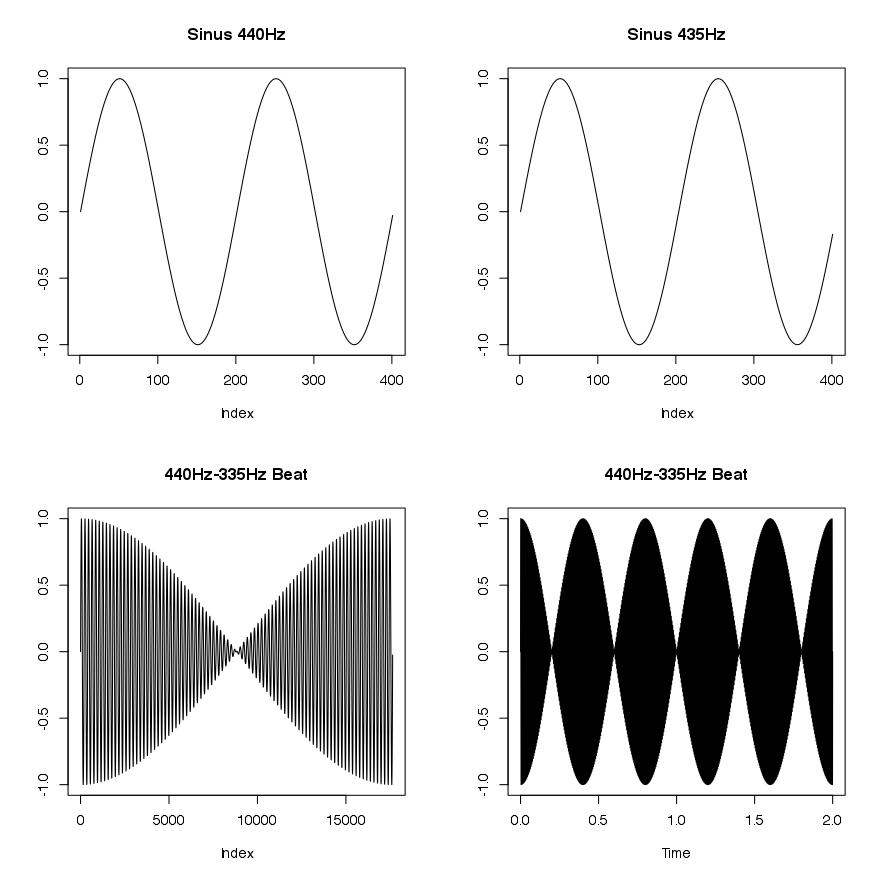
The following graphic shows two almost similar sinus waves, one at 440 Hz and one slightly below, at 435 Hz. The sound data is produced for exactly 2 seconds of time at a 44100 Hz sample rate, giving us 88200 sample points for 2 seconds. The first three demonstrations of the graph show only the beginning of the wave whereas the last one presents the combination of both signals for the complete 2 seconds.
Basically a combination of two sinus waves can be mathematically represented by:
![]() And if we assume that both amplitudes are the same we get the reduced form by:
And if we assume that both amplitudes are the same we get the reduced form by:
![]()
It is interesting to understand that the resulting frequency of the beat, i.e. the recognized periodic fluctuation of volume, is given by:
![]()
440Hz – Sinus – 2 seconds
435Hz – Sinus – 2 seconds
435 & 440Hz – Sinus – resulting beat frequency – 2 seconds
The oscillations in this post are simple created in R by using standard mathematical functions in combination with the time series package in R. In addition the seewave package is used to store the sinus waves as a .wav file to the system.
|
1 2 |
install.packages("seewave") require("seewave") |
The time series package handles data as equispaced points in time. This is in accordance with the sampling of continuous sound signals as the become digitized. A common used sampling frequency for CD quality is 44.1 kHz which results in 88.2k sample points for a length of 2 seconds.
|
1 2 3 4 5 6 7 8 9 10 11 12 13 14 15 |
s1<-sin(2*pi*440*seq(0,2,length.out=88200)) s1<-ts(data=s1, start=0, frequency=44100) jpeg(filename = "440Hz Sinus.jpg", width=880,height=880,res=100) plot(head(s1,401),type="l",ylab="") dev.off() s2<-sin(2*pi*435*seq(0,2,length.out=88200)) s2<-ts(data=s2, start=0, frequency=44100) jpeg(filename = "435Hz Sinus.jpg", width=880,height=880,res=100) plot(head(s2,401),type="l",ylab="") dev.off() s3<-(s1+s2)/2 |
For ease of use the summation of the amplitude 2a becomes reduced to a by division.
|
1 2 3 4 |
f<-44100 savewav(s1,f=f ,filename = "s1.wav") savewav(s2,f=f ,filename = "s2.wav") savewav(s3,f=f ,filename = "s3.wav") |
The graphical representation of the sound can easily be saved as a .jpg file to the system.
|
1 2 3 4 5 6 7 |
jpeg(filename = "435Hz-440Hz-beatsfrequency-4plots.jpg", width=880,height=880,res=100) par(mfrow=c(2,2)) plot(head(s1,401),type="l",ylab="",main="Sinus 440Hz") plot(head(s2,401),type="l",ylab="",main="Sinus 435Hz") plot(head(s3,17640),type="l",ylab="",main="440Hz-335Hz Beat") plot(s3,type="l",ylab="",main="440Hz-335Hz Beat") dev.off() |
In addition to the sample above we can also see and hear what it is like when the beat effect fades out and the brain starts to recognize two different tones. Therefore the next few examples present the resulting wave after summing two different frequencies, where one is always 440 Hz.
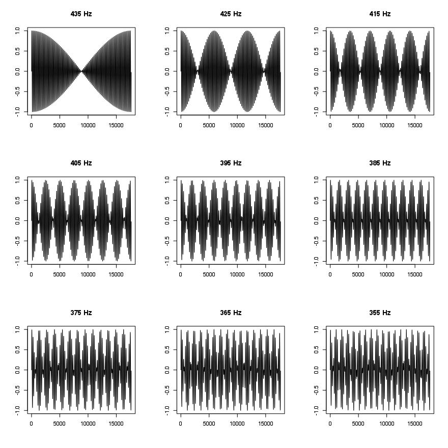
435 & 440Hz – Sinus – resulting beat frequency – 2 seconds
425 & 440Hz – Sinus – resulting (beat) frequency – 2 seconds
415 & 440Hz – Sinus – resulting (beat) frequency – 2 seconds
405 & 440Hz – Sinus – resulting (beat) frequency – 2 seconds
395 & 440Hz – Sinus – resulting (beat) frequency – 2 seconds
485 & 440Hz – Sinus – resulting (beat) frequency – 2 seconds
|
1 2 3 4 5 6 7 8 9 10 11 12 13 14 15 16 17 |
jpeg(filename = "beatsfrequency-9examples.jpg", width=880,height=880,res=100) par(mfrow=c(3,3)) for(i in 1:9){ e<-445-i*10 s1<-sin(2*pi*440*seq(0,2,length.out=88200)) s1<-ts(data=s1, start=0, frequency=44100) s2<-sin(2*pi*e*seq(0,2,length.out=88200)) s2<-ts(data=s2, start=0, frequency=44100) s3<-s1+s2 #jpeg(filename = "beatsfrequency.jpg", width=880,height=880,res=100) plot(head(s3/2,17640),type="l",ylab="",xlab="",main=paste(e,"Hz")) #plot(s3,type="l") #dev.off() f<-44100 savewav((s3/2),f=f ,filename = paste(e,"Hz - 440Hz-beat.wav")) } dev.off() |
- http://cran.r-project.org/web/views/TimeSeries.html
- http://cran.r-project.org/web/packages/seewave/index.html
Latex code for the Formulas above:
|
1 2 3 4 5 6 7 8 9 10 11 12 13 |
sin(2 \pi f_1t)+sin(2 \pi f_2t)=2sin(2 \pi \frac{f_1+f_2}{2} t)sin(2 \pi \frac{f_1-f_2}{2} t) x=(a_2-a_1)cos \omega_2t+2a_1cos\frac{\omega_1+\omega_2}{2}tcos\frac{\omega_2-\omega_1}{2}t x=2a_1cos\frac{\omega_1+\omega_2}{2}tcos\frac{\omega_2-\omega_1}{2}t \omega_a=\frac{\omega_1+\omega_2}{2} \omega_b=\frac{\omega_2-\omega_1}{2} \omega_s=\omega_2-\omega_1 f_s=f_2-f_1 |