Category Archives: Soundengineering

A day full of mixing.

03/15/2023Allgemein, Engineering, SoundengineeringMartin Stoppacher

ECR 2023

03/03/2023Allgemein, Engineering, SoundengineeringMartin Stoppacher

Some impressions from the ECR Congress 2023.

Engineering (FOH) at Starmania Tour 2021

09/28/2021Allgemein, Engineering, SoundengineeringMartin Stoppacher

Some Impressions from the Starmania Tour 2021. I operated the shows in Linz, Innsbruck and Vienna. It was a lot of fun to work with all the young talents at the show. 🙂

Kultur beim Winzer: Karl Ritter und Melissa Coleman @ Schloss Gobelsburg 2021

08/02/2021Allgemein, Engineering, SoundengineeringMartin Stoppacher

Some impressions from the “Kultur beim Winzer” shows in 2021. It was especially nice at “Schloss Gobelsburg” mixing the show in a wine cellar.

creating jukebox labels

08/22/2020Engineering, R, SoundengineeringMartin Stoppacher

# - - - - - - - - - - - - - - - - - - - - - - - - - - - - - - - - - - - - - - - #
# jukebox labels

j_list  <- read.csv2('Mappe1.csv', skip = 2)

j_list[ 1, ]

j_list[ , 1 ]
length( j_list[ , 1 ] )

ceiling( length( j_list[ , 1 ] ) / 8 )


g <- 1

for( f in 1:ceiling( length( j_list[ , 1 ] ) / 8 ) ) {

  jpeg( paste( "jukebox_" , f, ".jpg", sep = "") , width = 800, height = 800 )

  #jpeg("test2.jpg", width=800, height=800)

  #par( mar = rep( 1, 4 ), bg = "white")
  #par( mfrow = c( 1, 1 ), bg = "white")

  par( mfrow = c( 4, 2 ), bg = "white")

  print( g )
  
  #for( e in 1:8 ){
  for( e in g:(g+7) ){
  
    plot.new()
    plot.window(xlim = c(0, 800), ylim = c(0, 250))
    #lines(c(0, 800, 800, 0,0), c(0, 0, 250, 250,0), type = "l", lwd = 6, col = "red") # data frame with points to connect

    lines(c(0, 800), c(0, 0), type = "l", lwd = 6, col = "red")
    lines(c(0, 800), c(250, 250), type = "l", lwd = 6, col = "red")

    #lines(c(0, 100), c(131, 131), type = "l", lwd = 4, col = "red") 
    #lines(c(0, 100), c(129, 130), type = "l", lwd = 4, col = "red")
    #lines(c(0, 100), c(129, 129), type = "l", lwd = 4, col = "red")

    for(i in 119:131){ lines(c(0, 100), c(i, i), type = "l", lwd = 4, col = "red") }

    #lines(c(700, 800), c(123, 123), type = "l", lwd = 4, col = "red")
    #lines(c(700, 800), c(121, 121), type = "l", lwd = 4, col = "red")
    #lines(c(700, 800), c(119, 119), type = "l", lwd = 4, col = "red")

    for(i in 119:131){ lines(c(700, 800), c(i, i), type = "l", lwd = 4, col = "red") }

    #lines(c(0, 100, 100, 700,700,800), c(125, 125, 150, 150,125,125), type = "l", lwd = 7, col = "red") # data frame with points to connect
    #lines(c(0, 100, 100, 700,700,800), c(125, 125, 100, 100,125,125), type = "l", lwd = 7, col = "red") # data frame with points to connect

    #lines(c(100, 100, 100, 700,700,700), c(125, 125, 150, 150,125,125), type = "l", lwd = 7, col = "black") # data frame with points to connect
    #lines(c(100, 100, 100, 700,700,700), c(125, 125, 100, 100,125,125), type = "l", lwd = 7, col = "black") # data frame with points to connect

    #lines(c(100, 100, 100, 700,700,700), c(125, 125, 150, 150,125,125), type = "l", lwd = 3, col = "red") # data frame with points to connect
    #lines(c(100, 100, 100, 700,700,700), c(125, 125, 100, 100,125,125), type = "l", lwd = 3, col = "red") # data frame with points to connect

    lines(c(105, 105, 105, 695,695,695), c(125, 125, 150, 150,125,125), type = "l", lwd = 3, col = "red") # data frame with points to connect
    lines(c(105, 105, 105, 695,695,695), c(125, 125, 100, 100,125,125), type = "l", lwd = 3, col = "red") # data frame with points to connect

    c <- "black"
    f <- "Times New Roman"
    ce <- 2

    #text(400,125,"Rock",cex = 3, col = c, family=f)
    #text(400,200,"Side A",cex = 3, col = "Black")
    #text(400,50,"Side B",cex = 3, col = "Black")

    text( 400, 200, j_list[ e, 1 ], cex = ce, col = c, family = f )
    text( 400, 125, j_list[ e, 2 ] ,cex = ce, col = c, family = f )
    text( 400, 50, j_list[ e, 3 ], cex = ce, col = c, family = f )

  }

  g <- g + 8
  
  graphics.off()
  #browseURL("test.jpg")
  #browseURL("test2.jpg")
  #browseURL( paste( "jukebox_" , f, ".jpg", sep = "") )

}

# Martin Stoppacher                                                             #
# office@martinstoppacher.com                                                   #
# - - - - - - - - - - - - - - - - - - - - - - - - - - - - - - - - - - - - - - - #
#################################################################################

# - - - - - - - - - - - - - - - - - - - - - - - - - - - - - - - - - - - - - - - #

# jukebox labels

j_list <- read.csv2('Mappe1.csv', skip = 2)

j_list[ 1, ]

j_list[ , 1 ]

length( j_list[ , 1 ] )

ceiling( length( j_list[ , 1 ] ) / 8 )

g <- 1

for( f in 1:ceiling( length( j_list[ , 1 ] ) / 8 ) ) {

jpeg( paste( "jukebox_" , f, ".jpg", sep = "") , width = 800, height = 800 )

#jpeg("test2.jpg", width=800, height=800)

#par( mar = rep( 1, 4 ), bg = "white")

#par( mfrow = c( 1, 1 ), bg = "white")

par( mfrow = c( 4, 2 ), bg = "white")

print( g )

#for( e in 1:8 ){

for( e in g:(g+7) ){

plot.new()

plot.window(xlim = c(0, 800), ylim = c(0, 250))

#lines(c(0, 800, 800, 0,0), c(0, 0, 250, 250,0), type = "l", lwd = 6, col = "red") # data frame with points to connect

lines(c(0, 800), c(0, 0), type = "l", lwd = 6, col = "red")

lines(c(0, 800), c(250, 250), type = "l", lwd = 6, col = "red")

#lines(c(0, 100), c(131, 131), type = "l", lwd = 4, col = "red")

#lines(c(0, 100), c(129, 130), type = "l", lwd = 4, col = "red")

#lines(c(0, 100), c(129, 129), type = "l", lwd = 4, col = "red")

for(i in 119:131){ lines(c(0, 100), c(i, i), type = "l", lwd = 4, col = "red") }

#lines(c(700, 800), c(123, 123), type = "l", lwd = 4, col = "red")

#lines(c(700, 800), c(121, 121), type = "l", lwd = 4, col = "red")

#lines(c(700, 800), c(119, 119), type = "l", lwd = 4, col = "red")

for(i in 119:131){ lines(c(700, 800), c(i, i), type = "l", lwd = 4, col = "red") }

#lines(c(0, 100, 100, 700,700,800), c(125, 125, 150, 150,125,125), type = "l", lwd = 7, col = "red") # data frame with points to connect

#lines(c(0, 100, 100, 700,700,800), c(125, 125, 100, 100,125,125), type = "l", lwd = 7, col = "red") # data frame with points to connect

#lines(c(100, 100, 100, 700,700,700), c(125, 125, 150, 150,125,125), type = "l", lwd = 7, col = "black") # data frame with points to connect

#lines(c(100, 100, 100, 700,700,700), c(125, 125, 100, 100,125,125), type = "l", lwd = 7, col = "black") # data frame with points to connect

#lines(c(100, 100, 100, 700,700,700), c(125, 125, 150, 150,125,125), type = "l", lwd = 3, col = "red") # data frame with points to connect

#lines(c(100, 100, 100, 700,700,700), c(125, 125, 100, 100,125,125), type = "l", lwd = 3, col = "red") # data frame with points to connect

lines(c(105, 105, 105, 695,695,695), c(125, 125, 150, 150,125,125), type = "l", lwd = 3, col = "red") # data frame with points to connect

lines(c(105, 105, 105, 695,695,695), c(125, 125, 100, 100,125,125), type = "l", lwd = 3, col = "red") # data frame with points to connect

c <- "black"

f <- "Times New Roman"

ce <- 2

#text(400,125,"Rock",cex = 3, col = c, family=f)

#text(400,200,"Side A",cex = 3, col = "Black")

#text(400,50,"Side B",cex = 3, col = "Black")

text( 400, 200, j_list[ e, 1 ], cex = ce, col = c, family = f )

text( 400, 125, j_list[ e, 2 ] ,cex = ce, col = c, family = f )

text( 400, 50, j_list[ e, 3 ], cex = ce, col = c, family = f )

}

g <- g + 8

graphics.off()

#browseURL("test.jpg")

#browseURL("test2.jpg")

#browseURL( paste( "jukebox_" , f, ".jpg", sep = "") )

}

# Martin Stoppacher #

# office@martinstoppacher.com #

# - - - - - - - - - - - - - - - - - - - - - - - - - - - - - - - - - - - - - - - #

#################################################################################

Original:

Created:

Audio file conversion with afconvert (mac)

10/02/2017Code, Engineering, Programming, SoundengineeringMartin Stoppacher

I was looking for a simple and elegant way to convert a high amount of audio files from one format (.caf) to another (.aif). The solution i found is a very elegant one and also comes included with your operating system – if using a MAC.

afconvert -f AIFF -d BEI24@48000 "Wow Bass 03.caf" "Wow Bass 03.aif"

1	afconvert -f AIFF -d BEI24@48000 "Wow Bass 03.caf" "Wow Bass 03.aif"

And now here is the most amazing part. It is super easy to execute the conversion of multiple files by just one command line.

for i in *.caf; do afconvert -f AIFF -d BEI24@48000 "$i" "${i%.caf}.aif"; done

1	for i in *.caf; do afconvert -f AIFF -d BEI24@48000 "$i" "${i%.caf}.aif"; done

or to run through subdirectories:

for d in */ ; do cd $d; pwd; cd ..; done
for d in */ ; do cd $d; for i in *.caf; do echo *caf; pwd; done; cd ..; done;
for d in */ ; do cd $d; for i in *.caf; do afconvert -f AIFF -d BEI24@48000 "$i" "${i%.caf}.aif"; done; cd ..; done

for d in */ ; do cd $d; pwd; cd ..; done

for d in */ ; do cd $d; for i in *.caf; do echo *caf; pwd; done; cd ..; done;

for d in */ ; do cd $d; for i in *.caf; do afconvert -f AIFF -d BEI24@48000 "$i" "${i%.caf}.aif"; done; cd ..; done

or with recursion by using find:

find -name "*.caf"
find . -type f -iname '*.caf' -print | while read -r name; do cp "$name" "/.../..."; done
find . -type f -iname '*.caf' -print | while read -r name; do afconvert -f AIFF -d BEI24@48000 "$name" "/Volumes/Daten/Logic/test/${name%.*}.aif"; done

find -name "*.caf"

find . -type f -iname '*.caf' -print | while read -r name; do cp "$name" "/.../..."; done

find . -type f -iname '*.caf' -print | while read -r name; do afconvert -f AIFF -d BEI24@48000 "$name" "/Volumes/Daten/Logic/test/${name%.*}.aif"; done

Key	linear PCM format
LE	Little Endian
BE	Big Endian
F	Floating point
I	Integer
UI	Unsigned integer
8/16/24/32/64	Number of bits

Number of bits	Information Size
8	256
16	65536
24	16777216
32	4294967296
64	18446744073709551616

afconvert -hf

1	afconvert -hf

Audio file and data formats:	data_formats:
‘3gpp’ = 3GP Audio (.3gp)	‘Qclp’ ‘aac ‘ ‘aace’ ‘aach’ ‘aacl’ ‘aacp’ ‘samr’
‘3gp2’ = 3GPP-2 Audio (.3g2)	Qclp’ ‘aac ‘ ‘aace’ ‘aach’ ‘aacl’ ‘aacp’ ‘samr’
‘adts’ = AAC ADTS (.aac, .adts)	‘aac ‘ ‘aach’ ‘aacp’
‘ac-3’ = AC3 (.ac3)	‘ac-3’
‘AIFC’ = AIFC (.aifc, .aiff, .aif)	I8 BEI16 BEI24 BEI32 BEF32 BEF64 UI8 ‘ulaw’ ‘alaw’ ‘MAC3’ ‘MAC6’ ‘ima4’ ‘QDMC’ ‘QDM2’ ‘Qclp’ ‘agsm’
‘AIFF’ = AIFF (.aiff, .aif)	I8 BEI16 BEI24 BEI32
‘amrf’ = AMR (.amr)	‘samr’
‘m4af’ = Apple MPEG-4 Audio (.m4a, .m4r)	‘aac ‘ ‘aace’ ‘aach’ ‘aacl’ ‘aacp’ ‘alac’
‘caff’ = CAF (.caf)	‘.mp1’ ‘.mp2’ ‘.mp3’ ‘QDM2’ ‘QDMC’ ‘Qclp’ ‘Qclq’ ‘aac ‘ ‘aace’ ‘aach’ ‘aacl’ ‘aacp’ ‘alac’ ‘alaw’ ‘dvi8’ ‘ilbc’ ‘ima4’ I8 BEI16 BEI24 BEI32 BEF32 BEF64 LEI16 LEI24 LEI32 LEF32 LEF64 ‘ms\x00\x02’ ‘ms\x00\x11’ ‘ms\x001’ ‘paac’ ‘samr’ ‘ulaw’
‘MPG1’ = MPEG Layer 1 (.mp1, .mpeg, .mpa)	‘.mp1’
‘MPG2’ = MPEG Layer 2 (.mp2, .mpeg, .mpa)	‘.mp2’
‘MPG3’ = MPEG Layer 3 (.mp3, .mpeg, .mpa)	‘.mp3’
‘mp4f’ = MPEG-4 Audio (.mp4)	data_formats: ‘aac ‘ ‘aace’ ‘aach’ ‘aacl’ ‘aacp’
‘NeXT’ = NeXT/Sun (.snd, .au)	I8 BEI16 BEI24 BEI32 BEF32 BEF64 ‘ulaw’
‘Sd2f’ = Sound Designer II (.sd2)	I8 BEI16 BEI24 BEI32
‘WAVE’ = WAVE (.wav)	UI8 LEI16 LEI24 LEI32 LEF32 LEF64 ‘ulaw’ ‘alaw’

Supported Audio File and Data Formats in OS X

My Sounds (Freesound.org)

01/31/2016Allgemein, Engineering, SoundengineeringMartin Stoppacher

This is a collection of my sounds at freesound.org. I try to keep the list up to date but sometimes there are more sounds available on freesound therefore please check out my freesound account and freesound in general. “Freesound is a collaborative database of Creative Commons Licensed sounds. Browse, download and share sounds.” – freesound.org

Support this Blog

Creating sounds out of financial data.

04/09/2015Allgemein, Code, Data Analysis, Engineering, Programming, R, Soundengineering, StatisticsMartin Stoppacher

# - - - - - - - - - - - - - - - - - - - - - - - - - - - - - - - - - - - - - - - - - - - #
#

install.packages("seewave")
require("seewave")
install.packages("tuneR")
require("tuneR")

#rm(list = ls(all = TRUE)) # clear current workspace #
setwd("/Users/martinstoppacher/R Analysis/3_Index Sounds/")

library("quantmod")

getSymbols("^GSPC",from=1900)

head(GSPC)

tail(GSPC)

jpeg(filename = "SP500.jpg1975-2015.jpg", width=880,height=880,res=100)
plot(Cl(GSPC),main="S&amp;P 500 Index (closing prices)")
dev.off()

summary(Cl(GSPC))

jpeg(filename = "SP500.jpg1975-1985.jpg", width=880,height=880,res=100)
plot(Cl(GSPC)["1975/1985"],main="S&amp;P 500 Index 1975-1985 (closing prices)")
dev.off()

jpeg(filename = "SP500.jpg1985-1995.jpg", width=880,height=880,res=100)
plot(Cl(GSPC)["1985/1995"],main="S&amp;P 500 Index 1985-1995 (closing prices)")
dev.off()

jpeg(filename = "SP500.jpg1995-2005.jpg", width=880,height=880,res=100)
plot(Cl(GSPC)["1995/2005"],main="S&amp;P 500 Index 1995-2005 (closing prices)")
dev.off()

jpeg(filename = "SP500.jpg2005-2015.jpg", width=880,height=880,res=100)
plot(Cl(GSPC)["2005/2015"],main="S&amp;P 500 Index 2005-2015 (closing prices)")
dev.off()

jpeg(filename = "SP500.jpg 1975-2005 4decades-new.jpg", width=880,height=880,res=100)
plot(as.numeric(Cl(GSPC)["1975/1984"]),main="S&amp;P 500 Index 1975-1985 - 4 decades (closing prices)",ylim=c(0,2100),type="l",ylab="index values",xlab="days (10 year)")
lines(as.numeric(Cl(GSPC)["1985/1994"]),col="red")
lines(as.numeric(Cl(GSPC)["1995/2004"]),col="blue")
lines(as.numeric(Cl(GSPC)["2005/2015"]),col="green")
legend("topleft", legend = c("1975-1984","1985-1994","1995-2004","2005-2014") , lty = 1, col = c("black","red","blue","green"))
dev.off()

jpeg(filename = "SP500.jpg 1975-2005 4decades percent-new2.jpg", width=880,height=880,res=100)
plot((as.numeric(Cl(GSPC)["1975/1984"])/as.numeric(Cl(GSPC)["1975/1984"][1])-1),main="S&amp;P 500 Index 1975-1985 - 4 decades (percent changes)",ylim=c(-0.4,2.3),type="l",ylab="index values",xlab="days (10 year)")
lines((as.numeric(Cl(GSPC)["1985/1994"])/as.numeric(Cl(GSPC)["1985/1994"][1])-1),col="red")
lines((as.numeric(Cl(GSPC)["1995/2004"])/as.numeric(Cl(GSPC)["1995/2004"][1])-1),col="blue")
lines((as.numeric(Cl(GSPC)["2005/2014"])/as.numeric(Cl(GSPC)["2005/2014"][1])-1),col="green")
legend("topleft", legend = c("1975-1984","1985-1994","1995-2004","2005-2014") , lty = 1, col = c("black","red","blue","green"))
dev.off()

jpeg(filename = "SP500.jpg 1975-2005 4otherdecades percent2-new.jpg", width=880,height=880,res=100)
plot(as.numeric(Cl(GSPC)["1980/1989"])/as.numeric(Cl(GSPC)["1980/1989"][1]),main="S&amp;P 500 Index 1975-2015 - new truncation - (percent changes)",ylim=c(0.6,4.2),type="l",ylab="index values",xlab="days (10 year)",col="yellow")
lines(as.numeric(Cl(GSPC)["1975/1979"])/as.numeric(Cl(GSPC)["1975/1979"][1]),col="red")
lines(as.numeric(Cl(GSPC)["1990/1999"])/as.numeric(Cl(GSPC)["1990/1999"][1]),col="black")
lines(as.numeric(Cl(GSPC)["2000/2009"])/as.numeric(Cl(GSPC)["2000/2009"][1]),col="blue")
lines(as.numeric(Cl(GSPC)["2010/2014"])/as.numeric(Cl(GSPC)["2010/2014"][1]),col="green")
legend("topleft", legend = c("1975-1979","1980-1989","1990-1999","2000-2009","2010-2014") , lty = 1, col = c("red","yellow","black","blue","green"))
dev.off()

library("PerformanceAnalytics")

Cl(GSPC)["2010/2015"]/as.numeric(Cl(GSPC)["2005/2015"][1])
charts.PerformanceSummary(,main="",xlab="")

# percent

jpeg(filename = "SP500.jpg1975-1985-percent.jpg", width=880,height=880,res=100)
plot(Cl(GSPC)["1975/1985"]/as.numeric(Cl(GSPC)["1975/1985"][1]),main="S&amp;P 500 Index 1975-1985 (closing prices)")
dev.off()

jpeg(filename = "SP500.jpg1985-1995-percent.jpg", width=880,height=880,res=100)
plot(Cl(GSPC)["1985/1995"]/as.numeric(Cl(GSPC)["1985/1995"][1]),main="S&amp;P 500 Index 1985-1995 (closing prices)")
dev.off()

jpeg(filename = "SP500.jpg1995-2005-percent.jpg", width=880,height=880,res=100)
plot(Cl(GSPC)["1995/2005"]/as.numeric(Cl(GSPC)["1995/2005"][1]),main="S&amp;P 500 Index 1995-2005 (closing prices)")
dev.off()

jpeg(filename = "SP500.jpg2005-2015-percent.jpg", width=880,height=880,res=100)
plot(Cl(GSPC)["2005/2015"]/as.numeric(Cl(GSPC)["2005/2015"][1]),main="S&amp;P 500 Index 2005-2015 (closing prices)")
dev.off()

GSPC.cl.close &lt;- diff(Cl(GSPC))
tail(GSPC.cl.close,20)
jpeg(filename = "SP500-first-difference-example.jpg", width=880,height=880,res=100)
plot(tail(GSPC.cl.close,200),main="S&amp;P 500 first difference")
dev.off()

##

GSPC.cl.close.roc &lt;- ROC(Cl(GSPC))
tail(GSPC.cl.close.roc,5)

#prices &lt;- Cl(GSPC) # ROC is log diff!
#log_returns &lt;- diff(log(prices), lag=1)
#tail(log_returns)

jpeg(filename = "SP500-first-roc-example.jpg", width=880,height=880,res=100)
plot(tail(GSPC.cl.close.roc,200),main="S&amp;P 500 first difference")
dev.off()

##

dax.roc &lt;- na.omit(ROC(Cl(GSPC)))*100
plot(head(dax.roc,20))
plot(dax.roc)

# standard

if(abs(max(dax.roc))&gt;abs(min(dax.roc))){
dax.roc.standard &lt;- as.numeric(dax.roc/max(dax.roc))
}else{
dax.roc.standard &lt;- as.numeric(dax.roc/abs(min(dax.roc)))
}

plot(dax.roc.standard,type="l")

w&lt;-dax.roc.standard
f=41000
savewav(w,f=f ,filename = "xyz.wav")
aw&lt;-readWave("xyz.wav")
play(aw)

f=10000
savewav(w,f=f ,filename = "xyz.wav")
aw&lt;-readWave("xyz.wav")
play(aw)

f=5000
savewav(w,f=f ,filename = "xyz.wav")
aw&lt;-readWave("xyz.wav")
play(aw)

dax.roc &lt;- as.numeric(dax.roc)
dax.roc2 &lt;- NULL
for(i in 1:length(dax.roc)){
dax.roc2 &lt;- rbind(dax.roc2,((dax.roc[i]+dax.roc[i+1])/2))
}
lines &lt;- NULL
for(i in 1:length(dax.roc)){
line &lt;- rbind(dax.roc[i],dax.roc2[i])
lines &lt;- rbind(lines,line)
}
dax.roc &lt;- na.omit(lines)
tail(dax.roc)

dax.roc &lt;- na.omit(ROC(SMA(Cl(GSPC),n=500)))*100
dax.roc &lt;- na.omit(ROC(Cl(GDAXI)))*100

dax.roc.standard &lt;- as.numeric(dax.roc/max(dax.roc))
dax.roc.standard &lt;- as.numeric(dax.roc/min(dax.roc))

hist(dax.roc.standard)

w&lt;-na.omit(SMA(dax.roc.standard,n=100))
w&lt;-dax.roc.standard

for(i in 1:5){
w&lt;-c(w,w)
}

f=32000
savewav(w,f=f ,filename = "xyz.wav")
aw&lt;-readWave("xyz.wav")
play(aw)

# Martin Stoppacher #
# office@martinstoppacher.com #
# - - - - - - - - - - - - - - - - - - - - - - - - - - - - - - - - - - - - - - - #
#################################################################################

100

101

102

103

104

105

106

107

108

109

110

111

112

113

114

115

116

117

118

119

120

121

122

123

124

125

126

127

128

129

130

131

132

133

134

135

136

137

138

139

140

141

142

143

144

145

146

147

148

149

150

151

152

153

154

155

156

157

158

159

160

161

162

163

164

165

166

167

168

169

170

171

172

173

174

175

176

177

# - - - - - - - - - - - - - - - - - - - - - - - - - - - - - - - - - - - - - - - - - - - #

install.packages("seewave")

require("seewave")

install.packages("tuneR")

require("tuneR")

#rm(list = ls(all = TRUE)) # clear current workspace #

setwd("/Users/martinstoppacher/R Analysis/3_Index Sounds/")

library("quantmod")

getSymbols("^GSPC",from=1900)

head(GSPC)

tail(GSPC)

jpeg(filename = "SP500.jpg1975-2015.jpg", width=880,height=880,res=100)

plot(Cl(GSPC),main="S&P 500 Index (closing prices)")

dev.off()

summary(Cl(GSPC))

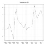
jpeg(filename = "SP500.jpg1975-1985.jpg", width=880,height=880,res=100)

plot(Cl(GSPC)["1975/1985"],main="S&P 500 Index 1975-1985 (closing prices)")

dev.off()

jpeg(filename = "SP500.jpg1985-1995.jpg", width=880,height=880,res=100)

plot(Cl(GSPC)["1985/1995"],main="S&P 500 Index 1985-1995 (closing prices)")

dev.off()

jpeg(filename = "SP500.jpg1995-2005.jpg", width=880,height=880,res=100)

plot(Cl(GSPC)["1995/2005"],main="S&P 500 Index 1995-2005 (closing prices)")

dev.off()

jpeg(filename = "SP500.jpg2005-2015.jpg", width=880,height=880,res=100)

plot(Cl(GSPC)["2005/2015"],main="S&P 500 Index 2005-2015 (closing prices)")

dev.off()

jpeg(filename = "SP500.jpg 1975-2005 4decades-new.jpg", width=880,height=880,res=100)

plot(as.numeric(Cl(GSPC)["1975/1984"]),main="S&P 500 Index 1975-1985 - 4 decades (closing prices)",ylim=c(0,2100),type="l",ylab="index values",xlab="days (10 year)")

lines(as.numeric(Cl(GSPC)["1985/1994"]),col="red")

lines(as.numeric(Cl(GSPC)["1995/2004"]),col="blue")

lines(as.numeric(Cl(GSPC)["2005/2015"]),col="green")

legend("topleft", legend = c("1975-1984","1985-1994","1995-2004","2005-2014") , lty = 1, col = c("black","red","blue","green"))

dev.off()

jpeg(filename = "SP500.jpg 1975-2005 4decades percent-new2.jpg", width=880,height=880,res=100)

plot((as.numeric(Cl(GSPC)["1975/1984"])/as.numeric(Cl(GSPC)["1975/1984"][1])-1),main="S&P 500 Index 1975-1985 - 4 decades (percent changes)",ylim=c(-0.4,2.3),type="l",ylab="index values",xlab="days (10 year)")

lines((as.numeric(Cl(GSPC)["1985/1994"])/as.numeric(Cl(GSPC)["1985/1994"][1])-1),col="red")

lines((as.numeric(Cl(GSPC)["1995/2004"])/as.numeric(Cl(GSPC)["1995/2004"][1])-1),col="blue")

lines((as.numeric(Cl(GSPC)["2005/2014"])/as.numeric(Cl(GSPC)["2005/2014"][1])-1),col="green")

legend("topleft", legend = c("1975-1984","1985-1994","1995-2004","2005-2014") , lty = 1, col = c("black","red","blue","green"))

dev.off()

jpeg(filename = "SP500.jpg 1975-2005 4otherdecades percent2-new.jpg", width=880,height=880,res=100)

plot(as.numeric(Cl(GSPC)["1980/1989"])/as.numeric(Cl(GSPC)["1980/1989"][1]),main="S&P 500 Index 1975-2015 - new truncation - (percent changes)",ylim=c(0.6,4.2),type="l",ylab="index values",xlab="days (10 year)",col="yellow")

lines(as.numeric(Cl(GSPC)["1975/1979"])/as.numeric(Cl(GSPC)["1975/1979"][1]),col="red")

lines(as.numeric(Cl(GSPC)["1990/1999"])/as.numeric(Cl(GSPC)["1990/1999"][1]),col="black")

lines(as.numeric(Cl(GSPC)["2000/2009"])/as.numeric(Cl(GSPC)["2000/2009"][1]),col="blue")

lines(as.numeric(Cl(GSPC)["2010/2014"])/as.numeric(Cl(GSPC)["2010/2014"][1]),col="green")

legend("topleft", legend = c("1975-1979","1980-1989","1990-1999","2000-2009","2010-2014") , lty = 1, col = c("red","yellow","black","blue","green"))

dev.off()

library("PerformanceAnalytics")

Cl(GSPC)["2010/2015"]/as.numeric(Cl(GSPC)["2005/2015"][1])

charts.PerformanceSummary(,main="",xlab="")

# percent

jpeg(filename = "SP500.jpg1975-1985-percent.jpg", width=880,height=880,res=100)

plot(Cl(GSPC)["1975/1985"]/as.numeric(Cl(GSPC)["1975/1985"][1]),main="S&P 500 Index 1975-1985 (closing prices)")

dev.off()

jpeg(filename = "SP500.jpg1985-1995-percent.jpg", width=880,height=880,res=100)

plot(Cl(GSPC)["1985/1995"]/as.numeric(Cl(GSPC)["1985/1995"][1]),main="S&P 500 Index 1985-1995 (closing prices)")

dev.off()

jpeg(filename = "SP500.jpg1995-2005-percent.jpg", width=880,height=880,res=100)

plot(Cl(GSPC)["1995/2005"]/as.numeric(Cl(GSPC)["1995/2005"][1]),main="S&P 500 Index 1995-2005 (closing prices)")

dev.off()

jpeg(filename = "SP500.jpg2005-2015-percent.jpg", width=880,height=880,res=100)

plot(Cl(GSPC)["2005/2015"]/as.numeric(Cl(GSPC)["2005/2015"][1]),main="S&P 500 Index 2005-2015 (closing prices)")

dev.off()

GSPC.cl.close <- diff(Cl(GSPC))

tail(GSPC.cl.close,20)

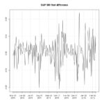
jpeg(filename = "SP500-first-difference-example.jpg", width=880,height=880,res=100)

plot(tail(GSPC.cl.close,200),main="S&P 500 first difference")

dev.off()

GSPC.cl.close.roc <- ROC(Cl(GSPC))

tail(GSPC.cl.close.roc,5)

#prices <- Cl(GSPC) # ROC is log diff!

#log_returns <- diff(log(prices), lag=1)

#tail(log_returns)

jpeg(filename = "SP500-first-roc-example.jpg", width=880,height=880,res=100)

plot(tail(GSPC.cl.close.roc,200),main="S&P 500 first difference")

dev.off()

dax.roc <- na.omit(ROC(Cl(GSPC)))*100

plot(head(dax.roc,20))

plot(dax.roc)

# standard

if(abs(max(dax.roc))>abs(min(dax.roc))){

dax.roc.standard <- as.numeric(dax.roc/max(dax.roc))

}else{

dax.roc.standard <- as.numeric(dax.roc/abs(min(dax.roc)))

}

plot(dax.roc.standard,type="l")

w<-dax.roc.standard

f=41000

savewav(w,f=f ,filename = "xyz.wav")

aw<-readWave("xyz.wav")

play(aw)

f=10000

savewav(w,f=f ,filename = "xyz.wav")

aw<-readWave("xyz.wav")

play(aw)

f=5000

savewav(w,f=f ,filename = "xyz.wav")

aw<-readWave("xyz.wav")

play(aw)

dax.roc <- as.numeric(dax.roc)

dax.roc2 <- NULL

for(i in 1:length(dax.roc)){

dax.roc2 <- rbind(dax.roc2,((dax.roc[i]+dax.roc[i+1])/2))

}

lines <- NULL

for(i in 1:length(dax.roc)){

line <- rbind(dax.roc[i],dax.roc2[i])

lines <- rbind(lines,line)

}

dax.roc <- na.omit(lines)

tail(dax.roc)

dax.roc <- na.omit(ROC(SMA(Cl(GSPC),n=500)))*100

dax.roc <- na.omit(ROC(Cl(GDAXI)))*100

dax.roc.standard <- as.numeric(dax.roc/max(dax.roc))

dax.roc.standard <- as.numeric(dax.roc/min(dax.roc))

hist(dax.roc.standard)

w<-na.omit(SMA(dax.roc.standard,n=100))

w<-dax.roc.standard

for(i in 1:5){

w<-c(w,w)

}

f=32000

savewav(w,f=f ,filename = "xyz.wav")

aw<-readWave("xyz.wav")

play(aw)

# Martin Stoppacher #

# office@martinstoppacher.com #

# - - - - - - - - - - - - - - - - - - - - - - - - - - - - - - - - - - - - - - - #

#################################################################################

Creating a beat frequency interference with R

02/23/2015Engineering, Programming, R, SoundengineeringMartin Stoppacher

A beat frequency is a mix of two frequencies which are very close to each other but not similar. The trick is that they are to close to each other to be separated by the human ear as two distinct frequencies, thus generating a single tone with fluctuating amplitude behavior – a periodic change in volume. In Fact this effect just appears within the human brain, therefore the two tones can be measured physically by using the appropriate instruments. Further more the effect also works in a binaural situation where one ear can only hear one frequency respectively.

The following graphic shows two almost similar sinus waves, one at 440 Hz and one slightly below, at 435 Hz. The sound data is produced for exactly 2 seconds of time at a 44100 Hz sample rate, giving us 88200 sample points for 2 seconds. The first three demonstrations of the graph show only the beginning of the wave whereas the last one presents the combination of both signals for the complete 2 seconds.

435Hz-440Hz-beatsfrequency-4plots

Basically a combination of two sinus waves can be mathematically represented by:

And if we assume that both amplitudes are the same we get the reduced form by:

It is interesting to understand that the resulting frequency of the beat, i.e. the recognized periodic fluctuation of volume, is given by:

440Hz – Sinus – 2 seconds

435Hz – Sinus – 2 seconds

435 & 440Hz – Sinus – resulting beat frequency – 2 seconds

The oscillations in this post are simple created in R by using standard mathematical functions in combination with the time series package in R. In addition the seewave package is used to store the sinus waves as a .wav file to the system.

install.packages("seewave")
require("seewave")

1 2	install.packages("seewave") require("seewave")

The time series package handles data as equispaced points in time. This is in accordance with the sampling of continuous sound signals as the become digitized. A common used sampling frequency for CD quality is 44.1 kHz which results in 88.2k sample points for a length of 2 seconds.

s1<-sin(2*pi*440*seq(0,2,length.out=88200))
s1<-ts(data=s1, start=0, frequency=44100)

jpeg(filename = "440Hz Sinus.jpg", width=880,height=880,res=100)
plot(head(s1,401),type="l",ylab="")
dev.off()

s2<-sin(2*pi*435*seq(0,2,length.out=88200))
s2<-ts(data=s2, start=0, frequency=44100)

jpeg(filename = "435Hz Sinus.jpg", width=880,height=880,res=100)
plot(head(s2,401),type="l",ylab="")
dev.off()

s3<-(s1+s2)/2

s1<-sin(2*pi*440*seq(0,2,length.out=88200))

s1<-ts(data=s1, start=0, frequency=44100)

jpeg(filename = "440Hz Sinus.jpg", width=880,height=880,res=100)

plot(head(s1,401),type="l",ylab="")

dev.off()

s2<-sin(2*pi*435*seq(0,2,length.out=88200))

s2<-ts(data=s2, start=0, frequency=44100)

jpeg(filename = "435Hz Sinus.jpg", width=880,height=880,res=100)

plot(head(s2,401),type="l",ylab="")

dev.off()

s3<-(s1+s2)/2

For ease of use the summation of the amplitude 2a becomes reduced to a by division.

f<-44100
savewav(s1,f=f ,filename = "s1.wav")
savewav(s2,f=f ,filename = "s2.wav")
savewav(s3,f=f ,filename = "s3.wav")

f<-44100

savewav(s1,f=f ,filename = "s1.wav")

savewav(s2,f=f ,filename = "s2.wav")

savewav(s3,f=f ,filename = "s3.wav")

The graphical representation of the sound can easily be saved as a .jpg file to the system.

jpeg(filename = "435Hz-440Hz-beatsfrequency-4plots.jpg", width=880,height=880,res=100)
par(mfrow=c(2,2))
plot(head(s1,401),type="l",ylab="",main="Sinus 440Hz")
plot(head(s2,401),type="l",ylab="",main="Sinus 435Hz")
plot(head(s3,17640),type="l",ylab="",main="440Hz-335Hz Beat")
plot(s3,type="l",ylab="",main="440Hz-335Hz Beat")
dev.off()

jpeg(filename = "435Hz-440Hz-beatsfrequency-4plots.jpg", width=880,height=880,res=100)

par(mfrow=c(2,2))

plot(head(s1,401),type="l",ylab="",main="Sinus 440Hz")

plot(head(s2,401),type="l",ylab="",main="Sinus 435Hz")

plot(head(s3,17640),type="l",ylab="",main="440Hz-335Hz Beat")

plot(s3,type="l",ylab="",main="440Hz-335Hz Beat")

dev.off()

In addition to the sample above we can also see and hear what it is like when the beat effect fades out and the brain starts to recognize two different tones. Therefore the next few examples present the resulting wave after summing two different frequencies, where one is always 440 Hz.

beatsfrequency-9examples

435 & 440Hz – Sinus – resulting beat frequency – 2 seconds

425 & 440Hz – Sinus – resulting (beat) frequency – 2 seconds

415 & 440Hz – Sinus – resulting (beat) frequency – 2 seconds

405 & 440Hz – Sinus – resulting (beat) frequency – 2 seconds

395 & 440Hz – Sinus – resulting (beat) frequency – 2 seconds

485 & 440Hz – Sinus – resulting (beat) frequency – 2 seconds

jpeg(filename = "beatsfrequency-9examples.jpg", width=880,height=880,res=100)
par(mfrow=c(3,3))
for(i in 1:9){
e<-445-i*10
s1<-sin(2*pi*440*seq(0,2,length.out=88200))
s1<-ts(data=s1, start=0, frequency=44100)
s2<-sin(2*pi*e*seq(0,2,length.out=88200))
s2<-ts(data=s2, start=0, frequency=44100)
s3<-s1+s2
#jpeg(filename = "beatsfrequency.jpg", width=880,height=880,res=100)
plot(head(s3/2,17640),type="l",ylab="",xlab="",main=paste(e,"Hz"))
#plot(s3,type="l")
#dev.off()
f<-44100
savewav((s3/2),f=f ,filename = paste(e,"Hz - 440Hz-beat.wav"))
}
dev.off()

jpeg(filename = "beatsfrequency-9examples.jpg", width=880,height=880,res=100)

par(mfrow=c(3,3))

for(i in 1:9){

e<-445-i*10

s1<-sin(2*pi*440*seq(0,2,length.out=88200))

s1<-ts(data=s1, start=0, frequency=44100)

s2<-sin(2*pi*e*seq(0,2,length.out=88200))

s2<-ts(data=s2, start=0, frequency=44100)

s3<-s1+s2

#jpeg(filename = "beatsfrequency.jpg", width=880,height=880,res=100)

plot(head(s3/2,17640),type="l",ylab="",xlab="",main=paste(e,"Hz"))

#plot(s3,type="l")

#dev.off()

f<-44100

savewav((s3/2),f=f ,filename = paste(e,"Hz - 440Hz-beat.wav"))

}

dev.off()

http://cran.r-project.org/web/views/TimeSeries.html
http://cran.r-project.org/web/packages/seewave/index.html

Latex code for the Formulas above:

sin(2 \pi f_1t)+sin(2 \pi f_2t)=2sin(2 \pi \frac{f_1+f_2}{2} t)sin(2 \pi \frac{f_1-f_2}{2} t)

x=(a_2-a_1)cos \omega_2t+2a_1cos\frac{\omega_1+\omega_2}{2}tcos\frac{\omega_2-\omega_1}{2}t

x=2a_1cos\frac{\omega_1+\omega_2}{2}tcos\frac{\omega_2-\omega_1}{2}t

\omega_a=\frac{\omega_1+\omega_2}{2}

\omega_b=\frac{\omega_2-\omega_1}{2}

\omega_s=\omega_2-\omega_1

f_s=f_2-f_1

sin(2 \pi f_1t)+sin(2 \pi f_2t)=2sin(2 \pi \frac{f_1+f_2}{2} t)sin(2 \pi \frac{f_1-f_2}{2} t)

x=(a_2-a_1)cos \omega_2t+2a_1cos\frac{\omega_1+\omega_2}{2}tcos\frac{\omega_2-\omega_1}{2}t

x=2a_1cos\frac{\omega_1+\omega_2}{2}tcos\frac{\omega_2-\omega_1}{2}t

\omega_a=\frac{\omega_1+\omega_2}{2}

\omega_b=\frac{\omega_2-\omega_1}{2}

\omega_s=\omega_2-\omega_1

f_s=f_2-f_1

Mixing at 25hours Hotel Vienna 2014

10/02/2014Allgemein, Engineering, SoundengineeringMartin Stoppacher