Basic Commands and Statistics with R – 2 – probability distibutions. R Functions for the most common probability distibutions.
|
1 2 3 4 5 6 7 8 9 10 11 12 13 14 15 16 17 18 19 20 21 22 23 24 25 26 27 28 29 30 31 32 33 34 35 36 37 38 39 40 41 42 43 44 45 46 47 48 49 50 51 52 53 54 55 |
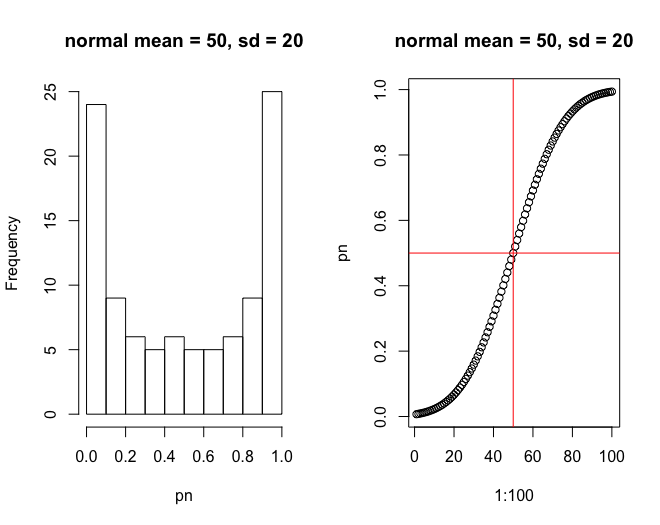
# - - - - - - - - - - - - - - - - - - - - - - - - - - - - - - - - - - - - - - - # # Basic Commands and Statistics with R - 2 - probability distibutions # An overview of the most common probability distibutions # eg: # https://en.wikipedia.org/wiki/List_of_probability_distributions # path: ~/ownCloud/STA_Statistics/Basic_Statistics/ # file_name: statistic_basics2.R # files_used: # - - - - - - - - - - - - - - - - - - - - - - - - - - - - - - - - - - - - - - - # # Probability Plots # Distribution Functions # # Normal pnorm qnorm dnorm rnorm # Beta pbeta qbeta dbeta rbeta # Binomial pbinom qbinom dbinom rbinom # Uniform punif qunif dunif runif # Cauchy pcauchy qcauchy dcauchy rcauchy # Chi-Square pchisq qchisq dchisq rchisq # Exponential pexp qexp dexp rexp # F pf qf df rf # Gamma pgamma qgamma dgamma rgamma # Geometric pgeom qgeom dgeom rgeom # Hypergeometric phyper qhyper dhyper rhyper # Logistic plogis qlogis dlogis rlogis # Log Normal plnorm qlnorm dlnorm rlnorm # Negative Binomial pnbinom qnbinom dnbinom rnbinom # Poisson ppois qpois dpois rpois # Student t pt qt dt rt # Studentized Range ptukey qtukey dtukey rtukey # Weibull pweibull qweibull dweibull rweibull # Wilcoxon Rank Sum Statistic pwilcox qwilcox dwilcox rwilcox # Wilcoxon Signed Rank Statistic psignrank qsignrank dsignrank rsignrank # ... # - - - - - - - - - - - - - - - - - - - - - - - - - - - - - - - - - - - - - - - # # Normal pnorm, qnorm, dnorm, rnorm # distribution function # direct - P ( X < 23.5 ) pn <- pnorm( 23.5, mean = 50, sd = 20 ) str( pn ) # num 0.0926 pn <- pnorm( 1:100, mean = 50, sd = 20 ) str( pn ) # num [1:100] 0.0512 0.0548 0.0586 0.0626 0.0668 ... par( mfrow = c( 1, 2 ) ) hist( pn, main = "normal mean = 50, sd = 20" ) plot( 1:100, pn, main = "normal mean = 50, sd = 20") abline( h = 0.5, v = 50, col = "red" ) par( mfrow = c( 1, 1 ) ) |
|
1 2 3 4 5 6 7 8 9 10 11 12 13 14 15 16 17 18 |
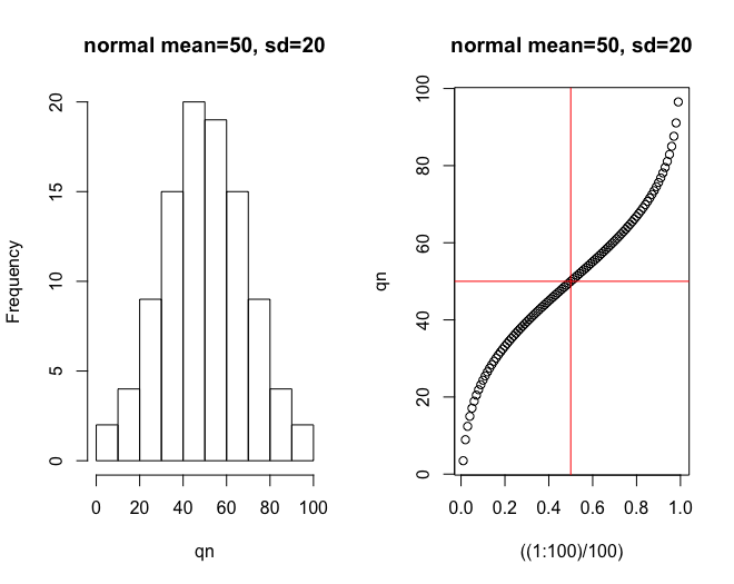
# quantile function # Inverse - qnorm looks up the p-th quantile of the normal distribution qn <- qnorm( 0.5, mean = 50, sd = 20 ) str( qn ) # num 50 qn <- qnorm( ( ( 1:100 ) / 100 ), mean = 50, sd = 20 ) str( qn ); qn; # [1] 3.47 8.93 12.38 14.99 17.10 18.90 20.48 21.90 23.18 24.37 25.47 26.5 #hist(qn,breaks=150) par( mfrow = c( 1, 2 ) ) hist( qn, main = "normal mean = 50, sd = 20" ) plot( ( ( 1:100 ) / 100 ), qn, main = "normal mean = 50, sd = 20" ) abline( v = 0.5, h = 50, col = "red" ) par( mfrow = c( 1, 1 ) ) |
|
1 2 3 4 5 6 7 8 |
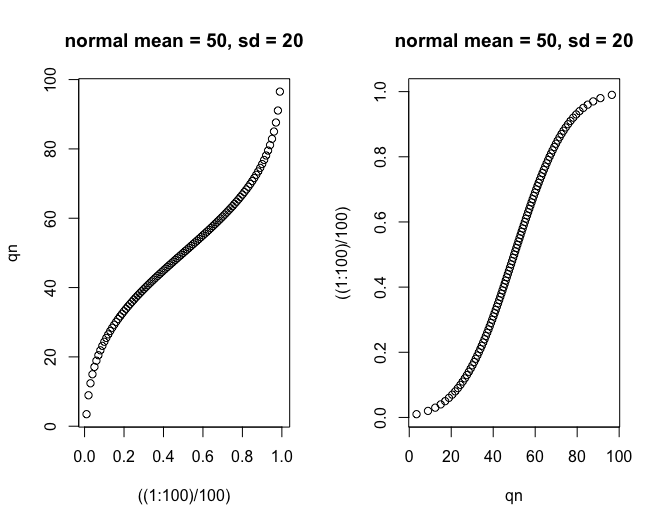
# invertet plot par( mfrow = c( 1, 2 ) ) plot( ( ( 1:100 ) / 100 ), qn, main = "normal mean = 50, sd = 20") abline( h = 150, col = "red" ) plot( qn, ( ( 1:100 ) / 100 ), main = "normal mean = 50, sd = 20") abline( v = 150, col = "red" ) |
|
1 2 3 4 5 6 7 8 9 10 11 12 13 14 15 16 17 18 19 20 21 22 23 24 25 26 27 28 29 30 31 32 |
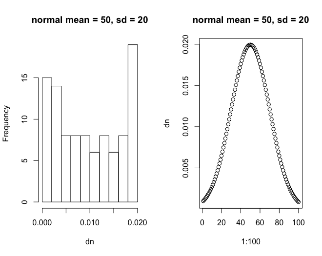
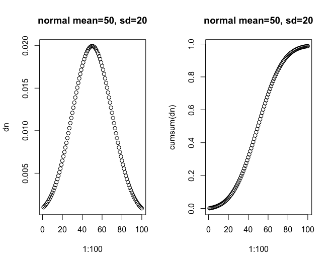
# Density function dn <- dnorm( 1:100, mean = 50, sd = 20) str( dn ) dn # [1] 0.00099187 0.00111973 0.00126091 0.00141635 0.00158698 0.00177373 # 0.00197750 0.00219918 0.00243960 0.00269955 0.00297974 0.00328079 # [13] 0.00360324 0.00394751 0.00431387 0.00470245 0.00511325 0.00554604 # 0.00600045 0.00647588 0.00697153 0.00748637 0.00801917 0.00856843 # [25] 0.00913245 0.00970930 0.01029681 0.01089261 0.01149411 0.01209854 # 0.01270295 0.01330426 0.01389924 0.01448458 0.01505687 0.01561270 # [37] 0.01614862 0.01666123 0.01714719 0.01760327 0.01802635 0.01841351 # 0.01876202 0.01906939 0.01933341 0.01955213 0.01972397 0.01984763 # [49] 0.01992220 0.01994711 0.01992220 0.01984763 0.01972397 0.01955213 # 0.01933341 0.01906939 0.01876202 0.01841351 0.01802635 0.01760327 # [61] 0.01714719 0.01666123 0.01614862 0.01561270 0.01505687 0.01448458 # 0.01389924 0.01330426 0.01270295 0.01209854 0.01149411 0.01089261 # [73] 0.01029681 0.00970930 0.00913245 0.00856843 0.00801917 0.00748637 # 0.00697153 0.00647588 0.00600045 0.00554604 0.00511325 0.00470245 # [85] 0.00431387 0.00394751 0.00360324 0.00328079 0.00297974 0.00269955 # 0.00243960 0.00219918 0.00197750 0.00177373 0.00158698 0.00141635 # [97] 0.00126091 0.00111973 0.00099187 0.00087642 sum( dn ) # [1] 0.98756 par( mfrow = c( 1, 2 ) ) hist( dn, main = "normal mean = 50, sd = 20" ) plot( 1:100, dn, main = "normal mean = 50, sd = 20" ) par( mfrow = c( 1, 1 ) ) |
|
1 2 3 4 5 6 7 8 9 10 11 12 13 14 15 16 17 18 19 20 21 22 23 24 25 |
cumsum(dn) # [1] 0.00099187 0.00211159 0.00337251 0.00478886 0.00637584 0.00814957 # 0.01012707 0.01232625 0.01476585 0.01746540 0.02044514 0.02372593 # [13] 0.02732917 0.03127668 0.03559054 0.04029300 0.04540624 0.05095229 # 0.05695274 0.06342862 0.07040014 0.07788652 0.08590568 0.09447411 # [25] 0.10360657 0.11331587 0.12361268 0.13450529 0.14599940 0.15809794 # 0.17080089 0.18410515 0.19800440 0.21248897 0.22754584 0.24315854 # [37] 0.25930716 0.27596839 0.29311558 0.31071885 0.32874520 0.34715870 # 0.36592072 0.38499011 0.40432352 0.42387565 0.44359962 0.46344725 # [49] 0.48336944 0.50331656 0.52323875 0.54308638 0.56281035 0.58236248 # 0.60169589 0.62076528 0.63952729 0.65794080 0.67596715 0.69357042 # [61] 0.71071761 0.72737884 0.74352746 0.75914015 0.77419702 0.78868160 # 0.80258085 0.81588511 0.82858806 0.84068660 0.85218071 0.86307331 # [73] 0.87337013 0.88307943 0.89221188 0.90078031 0.90879948 0.91628585 # 0.92325738 0.92973326 0.93573371 0.94127975 0.94639300 0.95109545 # [85] 0.95540932 0.95935683 0.96296007 0.96624086 0.96922060 0.97192015 # 0.97435975 0.97655893 0.97853643 0.98031016 0.98189714 0.98331349 # [97] 0.98457440 0.98569413 0.98668600 0.98756241 par( mfrow = c( 1, 2 ) ) plot( 1:100, dn, main = "normal mean=50, sd=20" ) plot( 1:100, cumsum( dn ), main= "normal mean=50, sd=20" ) par( mfrow = c( 1,1 ) ) |
|
1 2 3 4 5 6 7 8 9 10 11 |
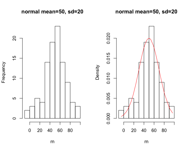
# Random generations - with specified normal distribution # random generation for the normal distribution rn <- rnorm( 100, mean = 50, sd = 20 ) par( mfrow=c( 1, 2 ) ) hist( rn, probability = FALSE, main = "normal mean = 50, sd = 20" ) hist( rn, probability = TRUE, main="normal mean = 50, sd = 20" ) #points( rn, dnorm( rn, mean = 50, sd = 20), col = "red" ) lines( sort( rn ), dnorm( sort( rn ), mean = 50, sd = 20 ), col= "red" ) par ( mfrow = c( 1, 1 ) ) |
|
1 2 3 4 5 6 7 8 9 10 11 12 13 14 15 16 17 18 19 20 |
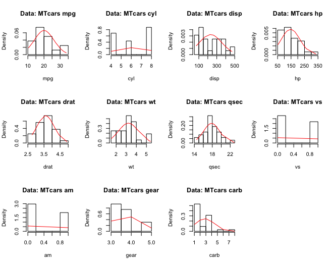
# - - - - - - - - - - - - - - - - - - - - - - - - - - - - - - - - - - - - - - - # # distributions for the mtcars data dnorm densities # https://stat.ethz.ch/R-manual/R-patched/library/datasets/html/mtcars.html attach( mtcars ) hist(mtcars$mpg, probability = TRUE) lines( sort( mtcars$mpg ), dnorm( sort( mtcars$mpg ) , mean = mean(mtcars$mpg) ,sd = sd(mtcars$mpg) ), col= "red" ) par( mfrow = c( 3, 4 ) ) for( i in 1:length( mtcars[1,] ) ){ hist( mtcars[,i], probability = TRUE, main = paste( "Data: MTcars", colnames( mtcars )[i] ), xlab = paste( colnames( mtcars )[i] ) ) lines( sort( mtcars[,i] ), dnorm( sort( mtcars[,i] ) , mean = mean( mtcars[,i] ) ,sd = sd( mtcars[,i] ) ), col= "red" ) } |
|
1 2 3 4 |
# Martin Stoppacher # # office@martinstoppacher.com # # - - - - - - - - - - - - - - - - - - - - - - - - - - - - - - - - - - - - - - - # ################################################################################# |