|
1 2 3 4 5 6 7 8 9 10 11 12 13 14 15 16 17 |
/* ***************************************************************************** */ /* Example of a syndication feed reader using the Project Rome API with */ /* BSF4ooRexx */ /* current version (2009) of Rome: rome1.0.jar https://rome.dev.java.net/ */ /* You need to implement this API plus the JDOM API */ /* jdom.jar , you can find this at https://jdom.org/ */ /* */ /* This class retrieves a syndfeed from the web by using a precreated */ /* Java class via BSF4ooRexx "com.sun.syndication.io.SyndFeedInput" methods */ /* created by Martin Stoppacher date: 26.12.2009 */ /* ***************************************************************************** */ javaclass = "FeedReader1" /* determine Java class to use */ get=.bsf~new(javaClass) /* create an instance of "javaClass" */ say get~getfeed /* calls the getfeed method in the FeedReader1 class */ ::requires BSF.CLS /* get the Java support */ |
Category Archives: Programming
Analyzing the World GDP Development using R
This is just a simple example of how to download and visualize data from the web by using the R-Project framework. Specifically data tables including GDP values from the world-bank data section are used which include absolute GDP per country data from 1980 to 2012.
http://data.worldbank.org/indicator/NY.GDP.MKTP.CD/countries/1W?display=default
There are 7 tables including 4 – 5 years of GDP data each. What this script does is to download each of this tables and merge it together into a single data frame which makes the data easily accessible for further analysis.
If we simply sum up all the single absolute GDP values per year we get the world GDP values for the period 1980 – 2012. The graphic below shows this development, measured in billions of USD.
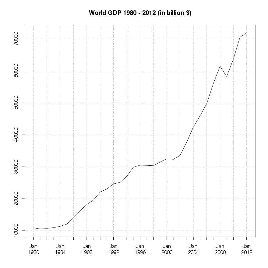

The similarity of the US output compared to the world GDP output is very obvious at first sight, showing the same setback in 2009 but no stagnation trough the 1998 – 2002 period. The fact that there is no setback in GDP output trough that period might indicate a week relationship between the financial turmoil in that time and the real economic output.
An other interesting fact is the growth of Chinas output, especially from 2002 onwards. This opens up the question on further resaerch on the reasons for this rapid growth and if some kind of regime switch occured turing that time . This rapid growth change lets China take the worlds second place, measured inabsolute GDP output, which makes China the second riches nation in the world, measured in absolute GDP value, from 2009 onwards.
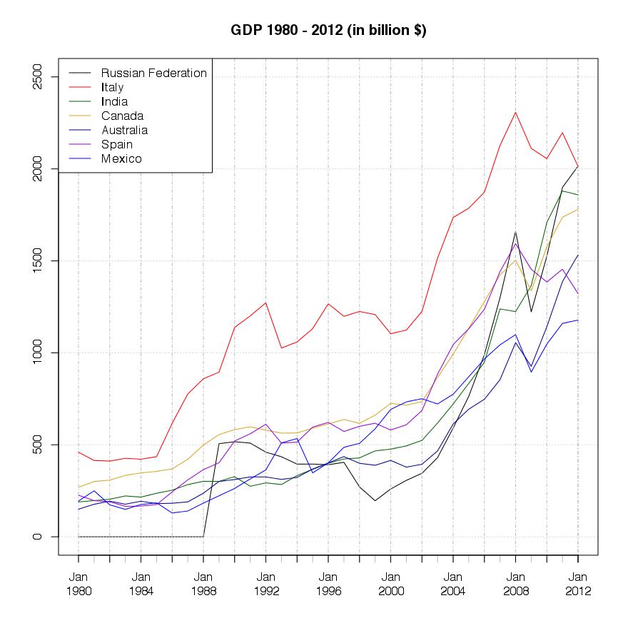
The last graphic is for the 8-14 ranked countries, measured by their absolute GDP USD value.
|
1 2 |
# - - - - - - - - - - - - - - - - - - - - - - - - - - - - - - - - - - - - - - - - # # Programming Part |
Ok, so here is the code:
|
1 2 3 4 5 6 7 8 9 |
# - - - - - - - - - - - - - - - - - - - - - - - - - - - - - - - - - - - - - - - - # # additional packages # install.packages("XML") # install.packages("gridExtra") library("XML") library("gridExtra") # - - - - - - - - - - - - - - - - - - - - - - - - - - - - - - - - - - - - - - - - # |
Basically i use two packages for these simple analytics. The “XML” packages is used to gather the data from the worldbank database and the “gridExtra” package is used for the graphical representation of a given dataset. The rest of the functionality already comes with the standard installation of the r-project software package.
The first step in the process is to download all the available data sets from the worldbank database and merge it together into one single data frame. This provides us with the opportunity of easy data handling. (Straight forward i just downloaded all the sets of data. Of course it would be possible to compress and automate this process by using loops, … , but i will try to cover this possibility at an other point here. As well as the automated gathering of data from different web sources, such as worldbank data, imf data, yahoo data, google data, quandl data, …)
|
1 2 3 4 5 6 7 8 9 10 11 12 13 14 15 16 17 18 19 20 21 22 23 24 25 26 27 28 29 30 31 32 33 34 |
# - - - - - - - - - - - - - - - - - - - - - - - - - - - - - - - - - - - - - - - - # # Download World GDP Data gdp6 <- readHTMLTable("http://data.worldbank.org/indicator/NY.GDP.MKTP.CD/countries/1W?display=default") gdp5 <- readHTMLTable("http://data.worldbank.org/indicator/NY.GDP.MKTP.CD/countries/1W?page=1&display=default") gdp4 <- readHTMLTable("http://data.worldbank.org/indicator/NY.GDP.MKTP.CD/countries/1W?page=2&display=default") gdp3 <- readHTMLTable("http://data.worldbank.org/indicator/NY.GDP.MKTP.CD/countries/1W?page=3&display=default") gdp2 <- readHTMLTable("http://data.worldbank.org/indicator/NY.GDP.MKTP.CD/countries/1W?page=4&display=default") gdp1 <- readHTMLTable("http://data.worldbank.org/indicator/NY.GDP.MKTP.CD/countries/1W?page=5&display=default") gdp <- readHTMLTable("http://data.worldbank.org/indicator/NY.GDP.MKTP.CD/countries/1W?page=6&display=default") gdp <- gdp[[1]] gdp <- as.data.frame(gdp) gdp.all <- gdp[,1:5] gdp1 <- gdp1[[1]] gdp1 <- as.data.frame(gdp1) gdp.all <- cbind(gdp.all,gdp1[,2:6]) # repeat that another 4 times gdp6 <- gdp6[[1]] gdp6 <- as.data.frame(gdp6) gdp.all <- cbind(gdp.all,gdp6[,2:5]) #save(gdp.all,file="gdp_all.R") # - - - - - - - - - - - - - - - - - - - - - - - - - - - - - - - - - - - - - - - - # |
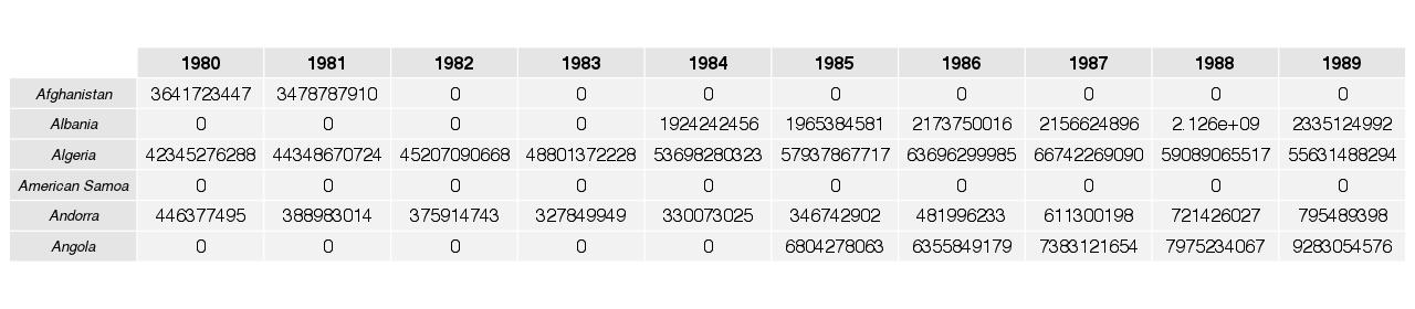
Once we gathered all the GDP data in one frame it is necessary to transform and clean some of the data. This is due to the fact that some of the cells in the data frame have no values (i.e. NA values in R) or they are in the wrong data formate (e.g. a character instead of numeric)
Basically we replace all NA values with a numerical 0, set all entries to numerical values and add the column names, which are the respective years of the data series, to the data frame.
|
1 2 3 4 5 6 7 8 9 10 11 12 13 14 15 16 17 18 19 20 21 22 23 24 25 26 27 28 29 30 31 |
# - - - - - - - - - - - - - - - - - - - - - - - - - - - - - - - - - - - - - - - - # # Data cleaning load("gdp_all.R") gdp.all.new <- data.frame() for(e in 1:length(gdp.all[,1])){ p<-NULL for(i in 2:length(gdp.all[1,])){ p[i-1]<-as.numeric(gsub(",","",gdp.all[e,i])) } p[is.na(p)]<-0 gdp.all.new<-rbind(gdp.all.new,p) } gdp.all.new <- cbind(as.character(gdp.all[,1]),gdp.all.new) colnames(gdp.all.new)<- c("Coutry","1980","1981","1982","1983","1984","1985","1986","1987","1988","1989","1990" ,"1991","1992","1993","1994","1995","1996","1997","1998","1999","2000","2001","2002" ,"2003","2004","2005","2006","2007","2008","2009","2010","2011","2012") rownames(gdp.all.new) <- as.character(gdp.all.new[,1]) gdp.all.new <- gdp.all.new[,2:34] jpeg(filename = "gdp_1980-2012_data.jpg", width=1280,height=280,res=100) grid.table(head(gdp.all.new[,1:10])) dev.off() #save(gdp.all.new,file="gdp_all_new.R") # - - - - - - - - - - - - - - - - - - - - - - - - - - - - - - - - - - - - - - - - # |
The results from this process can the seen in the plot below, which is a presentation of a part of the whole compiled table.
Output 1:
The next step is the graphical representation of the data which is the main goal of this short research. Therefore we apply the transpose function for the data frame and use the “xts” framework for time series handling and graphical output.
For the first plot (the cumulative world GDP) we have to process an other step before we can present the data. The single values for each country have to be summed up for each year to get the value for the world GDP of that specific year.
|
1 2 3 4 5 6 7 8 9 10 11 12 13 14 15 16 17 |
# - - - - - - - - - - - - - - - - - - - - - - - - - - - - - - - - - - - - - - - - # # Graphical representations load("gdp_all_new.R") gdp.all.new <- t(gdp.all.new) gdp.all.new.xts <-as.xts(gdp.all.new, order.by = as.Date(gsub(" ","-",paste(rownames(gdp.all.new),"01-01")), "%Y-%m-%d")) gdp.sum.new.xts <-as.xts(apply(gdp.all.new.xts,1,sum), order.by = as.Date(gsub(" ","-",paste(rownames(gdp.all.new),"01-01")), "%Y-%m-%d")) options(scipen=100) # Plot of the complete world GDP jpeg(filename = "gdp_1980-2012.jpg", width=880,height=880,res=100) plot(gdp.sum.new.xts/1000000000,type="l",main="World GDP 1980 - 2012 (in billion $)") dev.off() # - - - - - - - - - - - - - - - - - - - - - - - - - - - - - - - - - - - - - - - - # |
Output 2:
Plots for the top 7 countries measured in GDP value:
|
1 2 3 4 5 6 7 8 9 10 11 12 13 14 15 16 17 18 19 20 |
# - - - - - - - - - - - - - - - - - - - - - - - - - - - - - - - - - - - - - - - - # # Order Countries by GDP size top 7en gdp.all.new.xts.order <- gdp.all.new.xts[,order(gdp.all.new.xts[33,], decreasing = TRUE)] jpeg(filename = "gdp_1980-2012_top7.jpg", width=880,height=880,res=100) plot(gdp.all.new.xts.order[,1]/1000000000,type="l",main="GDP 1980 - 2012 (in billion $)",ylim=c(0,16000)) myColors <- c("black","red", "darkgreen", "goldenrod", "darkblue", "darkviolet","blue") for(i in 2:7){ lines(gdp.all.new.xts.order[,i]/1000000000, col = myColors[i]) } legend("topleft", legend = colnames(gdp.all.new.xts.order[,1:7]), lty = 1, col = myColors) dev.off() # - - - - - - - - - - - - - - - - - - - - - - - - - - - - - - - - - - - - - - - - # |
Output 3:
Plots for the top 8-14 countries measured in GDP value:
|
1 2 3 4 5 6 7 8 9 10 11 12 13 14 15 16 17 18 |
# - - - - - - - - - - - - - - - - - - - - - - - - - - - - - - - - - - - - - - - - # # Order Countries by GDP size top 8-14en jpeg(filename = "gdp_1980-2012_top8-14.jpg", width=880,height=880,res=100) plot(gdp.all.new.xts.order[,8]/1000000000,type="l",main="GDP 1980 - 2012 (in billion $)",ylim=c(0,2500)) myColors <- c("black","red", "darkgreen", "goldenrod", "darkblue", "darkviolet","blue") for(i in 9:14){ lines(gdp.all.new.xts.order[,i]/1000000000, col = myColors[i-7]) } legend("topleft", legend = colnames(gdp.all.new.xts.order[,8:14]), lty = 1, col = myColors) dev.off() # - - - - - - - - - - - - - - - - - - - - - - - - - - - - - - - - - - - - - - - - # |
Output 4:
– – – – – – – – – – – – – – – – – – – – – – – – – – – – – – – – – – – – – – – – – – – – – –
Please note that i do not always try to produce perfectly efficient code in a programming attitude but rather focus on the results and sociological, econometrical, … , insights gathered trough the process of data analytics.
If my focus especially belongs to coding i will try to catch that with an unique post, just for this specific topic. Nevertheless i strongly appreciate suggestions, additions and/or correction in both the analytical insights and the data analytical process and programming code.
– – – – – – – – – – – – – – – – – – – – – – – – – – – – – – – – – – – – – – – – – – – – – –
Data Source: data.worldbank.org/
– – – – – – – – – – – – – – – – – – – – – – – – – – – – – – – – – – – – – – – – – – – – – –
Martin Stoppacher, © 2014
Content syndication with the Project ROME Java API by using the open object scripting language ooRexx with BSF4ooRexx
Content syndication with the Project ROME Java API
by using the open object scripting language ooRexx
with BSF4ooRexx
–
Project Rome in combination with BSF4ooRexx
Martin Stoppacher
2010
Abstract
This text tries to convey a basic understanding and knowledge of concepts, usage and
possibilities of the “Project ROME”(1) (Java) API (2). Furthermore the text provides a description
and documentation about interfacing Java (and therefore the Project ROME API) with ooRexx (4)
by using its extension BSF4ooRexx.
Specifically the text deals with the functionalities Project ROME is providing, as well as its
technical concepts and relations. This functionalities get extended by using BSF4ooRexx and
therefore demonstrate how to use an external Java API in open object Rexx.
As Project ROME deals with the processing of content syndication (3) the first part of the paper
covers the explanation of concepts and basics related to content syndication.
The second part deals with the processing of content syndication via Project Rome by using the
Java programming language. Project Rome will be described and a few example programs in Java will explain its functionalities.
The following parts cover the usage of ooRexx (4) with BSF4ooRexx (5). Therefore a short
introduction to this topic will be given and afterwards the usage of Project Rome with
BSF4ooRexx will be explained through examples.
The final part is built by a collection of several example programs which demonstrate the usage of Project Rome. First some Java examples are shown and second the corresponding ooRexx examples demonstrate how it is possible to use the same classes within ooRexx.
An example of a syndication feed reader using the Project Rome API with BSF4ooRexx – “java.net.URL” feed reader (2_Rome.rxj)
|
1 2 3 4 5 6 7 8 9 10 11 12 13 14 15 16 17 18 19 20 21 22 23 24 25 26 27 28 29 30 31 32 33 34 35 36 |
/* ***************************************************************************** */ /* Example of a syndication feed reader using the Project Rome API with */ /* BSF4ooRexx */ /* current version (2009) of Rome: rome1.0.jar https://rome.dev.java.net/ */ /* You need to implement this API plus the JDOM API */ /* jdom.jar, you can find this at https://jdom.org/ */ /* This class retrieves a syndfeed from the web and prints some */ /* information about the feed using */ /* "com.sun.syndication.io.SyndFeedInput" methods */ /* created by Martin Stoppacher date: 26.12.2009 */ /* ***************************************************************************** */ say hello this reads a syndfeed --say please type in the url /* possible input statement for the feed URL */ --pull url --parse arg url /* optional input via arguments */ /* The url String is predefined in this example, to change the feed url */ /* replace to String in this file or use one of the above methods */ url= "http://rss.orf.at/fm4.xml" feedUrl=.bsf~new("java.net.URL", url) /* create an instance of java.net.URL */ say connecting__ || feedUrl~getAuthority() input=.bsf~new("com.sun.syndication.io.SyndFeedInput")/* creates a SyndFeedInput */ xmlr=.bsf~new("com.sun.syndication.io.XmlReader", feedUrl) /* Figures out the charset encoding of the XML document within the stream */ feed= input~build(xmlr) /* Builds a SyndFeedImpl from an Reader , also possible with SAX or DOM */ say bb~getDefaultEncoding() say feed /* returns the feed object */ ::requires BSF.cls /* get the Java support */ |
Syndication feed reader using the Project Rome API – (1_FeedReader.java)
|
1 2 3 4 5 6 7 8 9 10 11 12 13 14 15 16 17 18 19 20 21 22 23 24 25 26 27 28 29 30 31 32 33 34 35 36 37 38 39 40 41 42 43 44 45 46 47 48 49 50 51 52 53 54 55 56 57 58 59 60 61 62 |
/* ***************************************************************************** */ /* Example of a syndication feed reader using the Project Rome API */ /* current version of Rome: rome1.0.jar (2009) https://rome.dev.java.net/ */ /* You need to implement this API plus the JDOM API */ /* jdom.jar , you can find this at https://jdom.org/ */ /* Parts of this example are taken from the PRome Web Page tutorials */ /* https://rome.dev.java.net/ author: Alejandro Abdelnur */ /* */ /* This class retrieves a syndfeed from the web and prints its */ /* pure content to the system */ /* created by Martin Stoppacher date: 26.12.2009 */ /* ***************************************************************************** */ import java.net.URL; /* Class URL represents a Uniform Resource Locator, a pointer to a "resource" */ /* on the World Wide Web */ import java.io.InputStreamReader; /* An InputStreamReader is a bridge from byte streams to character streams */ import com.sun.syndication.feed.synd.SyndFeed; /* This is the Bean interface for all types of feeds. */ import com.sun.syndication.io.SyndFeedInput; /* Parses an XML document (File, InputStream, Reader, W3C SAX InputSource, W3C*/ /* DOM Document or JDom DOcument) into an WireFeed (RSS/Atom). */ import com.sun.syndication.io.XmlReader; /* Character stream that handles (or at least attemtps to) all the necessary */ /* Voodo to figure out the charset encoding of the XML document within */ /* the stream. */ public class 1_FeedReader { public static void main(String[] args) { boolean ok = false; if (args.length==1) { try { URL feedUrl = new URL(args[0]); /*creates a string with the URL*/ SyndFeedInput input = new SyndFeedInput(); /* new input object*/ SyndFeed feed = input.build(new XmlReader(feedUrl)); /* reads feed from URL and puts it into feed*/ System.out.println(feed); /* outputs file to system */ ok = true; } catch (Exception ex) { ex.printStackTrace(); System.out.println("ERROR: "+ex.getMessage()); } } if (!ok) { System.out.println(); System.out.println("FeedReader reads and prints any RSS/Atom feed type."); System.out.println("The first parameter must be the" +"URL of the feed to read."); System.out.println(); } } } |
- the Open Object Rexx (ooRexx) web site
- ROME is a set of RSS and Atom Utilities for Java
- Introduction to REXX and ooRexx – Flatscher Rony G.
- http://wi.wu-wien.ac.at:8002/rgf/
- http://wi.wu-wien.ac.at/rgf/diplomarbeiten/BakkStuff/2010/201001_Stoppacher/Project_Rome_in_combination_with_BSF4ooRexx_Presentation.pdf