Lately i was exploring the logistic map function because i was fascinated again how chaotic behavior can arise from very simple circumstances (i.e. a rather simple equation).
Of course, i learned about this in school but never got a chance to write some code.
So here it is. 🙂
And here is some of the code i wrote:
|
1 2 3 4 5 6 7 8 9 10 11 12 13 14 15 |
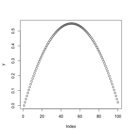
# - - - - - - - - - - - - - - - - - - - - - - - - - - - - - - - - - - - - - - - # # bifurcation tree, Logistic map # xn1=rxn(1-xn) rm(list = ls(all = TRUE)) r <- 2.2 # rate x <- 0.5 # population (r*x*(1-x)) r <- 2.2 (x <- seq(100,1)/100) y = r*x*(1-x) plot(y) |
|
1 2 3 4 5 6 7 8 9 10 11 12 13 |
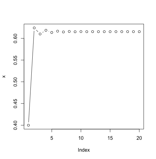
# - - - - - - - - - - - - - - - - - - - - - - - - - - - - - - - - - - - - - - - # # if the starting population is 0.1 r <- 2.6 x <- 0.1 for(i in 2:20){ (x[i] <- r*x[i-1]*(1-x[i-1])) print(i) print(x[i]) #Sys.sleep(0.5) } x plot(x, type="b") |
|
1 2 3 4 5 6 7 8 9 10 11 12 13 |
# - - - - - - - - - - - - - - - - - - - - - - - - - - - - - - - - - - - - - - - # # if the starting population is 0.8 r <- 2.6 x <- 0.8 for(i in 2:20){ (x[i] <- r*x[i-1]*(1-x[i-1])) print(i) print(x[i]) #Sys.sleep(0.5) } x plot(x, type="b") |

|
1 2 3 4 5 6 7 8 9 10 11 12 13 14 15 16 17 |
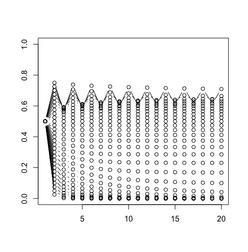
# - - - - - - - - - - - - - - - - - - - - - - - - - - - - - - - - - - - - - - - # # if we make variations to the initial population all of them stabilize plot(1:20,(1:20)/20,ylab="",xlab="",cex=0) for(e in ((1:9)/10)){ r <- 2.6 x <- e for(i in 2:20){ (x[i] <- r*x[i-1]*(1-x[i-1])) print(i) print(x[i]) #Sys.sleep(0.5) } x lines(x, type="b") } |

|
1 2 3 4 5 6 7 8 9 10 11 12 13 14 15 16 17 |
# - - - - - - - - - - - - - - - - - - - - - - - - - - - - - - - - - - - - - - - # # what does this look like if there are variations to the groth rate? plot(0,0, ylab="", xlab="", cex=0, xlim=c(1,20), ylim=c(0,1)) for(e in (1:30)/10){ r <- e x <- 0.5 for(i in 2:20){ (x[i] <- r*x[i-1]*(1-x[i-1])) print(i) print(x[i]) #Sys.sleep(0.5) } x lines(x, type="b") } |
|
1 2 3 4 5 6 7 8 9 10 11 12 13 14 15 16 17 18 19 |
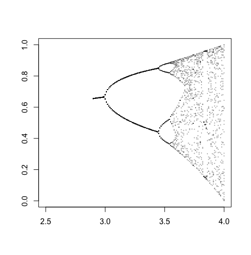
# - - - - - - - - - - - - - - - - - - - - - - - - - - - - - - - - - - - - - - - # # ploting more values but only the last plot(0,0, ylab="", xlab="", cex=0, xlim=c(2.5,4), ylim=c(0,1)) n<-300 m<-30 for(e in ((290:400)/100)){ print(r) r <- e x <- 0.1 for(i in 2:n){ (x[i] <- r*x[i-1]*(1-x[i-1])) print(r) print(x[i]) } x points(rep(r,(m+1)),x[(n-m):n], type="p", cex=0.2, lwd=0.2) } |
|
1 2 3 4 5 6 7 8 9 10 11 12 13 14 15 16 17 18 19 20 21 22 23 |
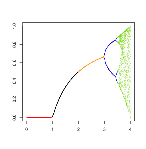
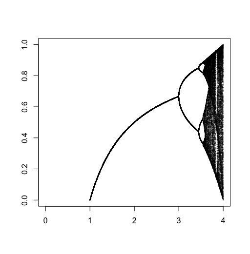
# - - - - - - - - - - - - - - - - - - - - - - - - - - - - - - - - - - - - - - - # # adding color plot(0,0, ylab="", xlab="", cex=0, xlim=c(0,4), ylim=c(0,1)) n<-100 m<-30 for(e in ((1:400)/100)){ print(r) r <- e x <- 0.6 for(i in 2:n){ (x[i] <- r*x[i-1]*(1-x[i-1])) print(r) print(x[i]) } x if(r<1)points(rep(r,(m+1)),x[(n-m):n], type="p", cex=0.2, lwd=0.2, col="red") if(r>=1&r<2)points(rep(r,(m+1)),x[(n-m):n], type="p", cex=0.2, lwd=0.2, col="black") if(r>=2&r<5)points(rep(r,(m+1)),x[(n-m):n], type="p", cex=0.2, lwd=0.2, col="orange") if(r>=3&r<=3.5)points(rep(r,(m+1)),x[(n-m):n], type="p", cex=0.2, lwd=0.2, col="blue") if(r>=3.5&r<=4)points(rep(r,(m+1)),x[(n-m):n], type="p", cex=0.2, lwd=0.2, col="green") } |
|
1 2 3 4 5 6 7 8 9 |
# - - - - - - - - - - - - - - - - - - - - - - - - - - - - - - - - - - - - - - - # # bifurcation tree as a function log.tree <- function(r=2, x=0.4, n=200){ for(i in 2:(n+1)){ (x[i] <- r*x[i-1]*(1-x[i-1])) } x <- x[2:(n+1)] } |
|
1 2 3 4 5 6 7 8 9 10 11 12 13 14 15 |
# - - - - - - - - - - - - - - - - - - - - - - - - - - - - - - - - - - - - - - - # # using the function with sapply point.count <- 50 # sets how many of the last observations to use r.seq <- seq(1,4,by=0.001) # a sequence for different rates plot(0,0, ylab="", xlab="", cex=0, xlim=c(0,4), ylim=c(0,1)) log.tree.points <- tail(sapply(r.seq, log.tree, x=0.1, n=3000),point.count) for(i in 1:length(r.seq)) points(rep(r.seq[i],point.count),log.tree.points[,i], cex=0.2, lwd=0.2) # - - - - - - - - - - - - - - - - - - - - - - - - - - - - - - - - - - - - - - - # # system.time(log.tree.points <- tail(sapply(r.seq, log.tree, x=0.1, n=300),point.count)) system.time(log.tree.points <- tail(sapply(r.seq, log.tree, x=0.1, n=3000),point.count)) system.time(log.tree.points <- tail(sapply(r.seq, log.tree, x=0.1, n=30000),point.count)) |
|
1 2 3 4 |
# Martin Stoppacher # # office@martinstoppacher.com # # - - - - - - - - - - - - - - - - - - - - - - - - - - - - - - - - - - - - - - - # ################################################################################# |