
All posts by Martin Stoppacher
Using trigonometric functions in R
R uses radiant as input for trigonometric functions.
|
1 2 3 4 5 6 7 |
# calculating rad pi/2 90*pi/180 # transforming degree into radiant degr<-c(0:360) degr rad<-grad*(pi/180) rad |
Now we can plot the function.
|
1 2 |
sin(rad) plot(sin(rad)) |
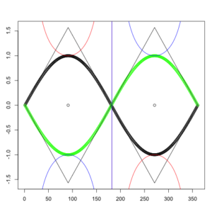
And by playing with the functions we get a funny graphic output.
|
1 2 3 4 5 6 7 8 9 |
plot(asin(sin(rad))) plot(asin(sin(rad)),type="l") points(sin(rad)) points(sin(rad)*-1,col="green") lines(asin(sin(rad))*-1) lines(1/sin(rad),col="red") lines(1/sin(rad)*-1,col="blue") points(x=91,y=0) points(x=271,y=0) |
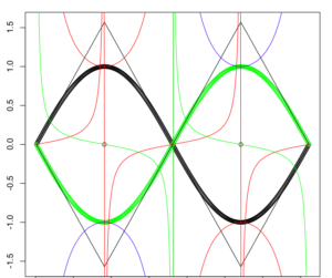
And if we include the tangent, the graphic looks like this:
|
1 2 3 4 5 6 7 |
tan(rad) tangens <- tan(rad) tangens[91]<-0 tangens[271]<-0 plot(tangens,type="l") lines(sin(rad),type="l",col="red") lines(cos(rad),type="l",col="green") |
|
1 2 3 4 5 |
lines(tangens,type="l",col="red") lines(1/tangens,type="l",col="green") # dividing by 10 for visual reasons lines(tangens/10,type="l",col="red") lines(1/tangens/10,type="l",col="green") |
|
1 2 3 4 |
plot(tangens,type="l") lines(1/tangens,type="l") plot(tangens,type="l") lines(1/tangens,type="l",col="green") |
Audio file conversion with afconvert (mac)
I was looking for a simple and elegant way to convert a high amount of audio files from one format (.caf) to another (.aif). The solution i found is a very elegant one and also comes included with your operating system – if using a MAC.
|
1 |
afconvert -f AIFF -d BEI24@48000 "Wow Bass 03.caf" "Wow Bass 03.aif" |
And now here is the most amazing part. It is super easy to execute the conversion of multiple files by just one command line.
|
1 |
for i in *.caf; do afconvert -f AIFF -d BEI24@48000 "$i" "${i%.caf}.aif"; done |
or to run through subdirectories:
|
1 2 3 |
for d in */ ; do cd $d; pwd; cd ..; done for d in */ ; do cd $d; for i in *.caf; do echo *caf; pwd; done; cd ..; done; for d in */ ; do cd $d; for i in *.caf; do afconvert -f AIFF -d BEI24@48000 "$i" "${i%.caf}.aif"; done; cd ..; done |
or with recursion by using find:
|
1 2 3 |
find -name "*.caf" find . -type f -iname '*.caf' -print | while read -r name; do cp "$name" "/.../..."; done find . -type f -iname '*.caf' -print | while read -r name; do afconvert -f AIFF -d BEI24@48000 "$name" "/Volumes/Daten/Logic/test/${name%.*}.aif"; done |
| Key | linear PCM format |
| LE | Little Endian |
| BE | Big Endian |
| F | Floating point |
| I | Integer |
| UI | Unsigned integer |
| 8/16/24/32/64 | Number of bits |
| Number of bits | Information Size |
| 8 | 256 |
| 16 | 65536 |
| 24 | 16777216 |
| 32 | 4294967296 |
| 64 | 18446744073709551616 |
|
1 |
afconvert -hf |
| Audio file and data formats: | data_formats: |
| ‘3gpp’ = 3GP Audio (.3gp) | ‘Qclp’ ‘aac ‘ ‘aace’ ‘aach’ ‘aacl’ ‘aacp’ ‘samr’ |
| ‘3gp2’ = 3GPP-2 Audio (.3g2) | Qclp’ ‘aac ‘ ‘aace’ ‘aach’ ‘aacl’ ‘aacp’ ‘samr’ |
| ‘adts’ = AAC ADTS (.aac, .adts) | ‘aac ‘ ‘aach’ ‘aacp’ |
| ‘ac-3’ = AC3 (.ac3) | ‘ac-3’ |
| ‘AIFC’ = AIFC (.aifc, .aiff, .aif) | I8 BEI16 BEI24 BEI32 BEF32 BEF64 UI8 ‘ulaw’ ‘alaw’ ‘MAC3’ ‘MAC6’ ‘ima4’ ‘QDMC’ ‘QDM2’ ‘Qclp’ ‘agsm’ |
| ‘AIFF’ = AIFF (.aiff, .aif) | I8 BEI16 BEI24 BEI32 |
| ‘amrf’ = AMR (.amr) | ‘samr’ |
| ‘m4af’ = Apple MPEG-4 Audio (.m4a, .m4r) | ‘aac ‘ ‘aace’ ‘aach’ ‘aacl’ ‘aacp’ ‘alac’ |
| ‘caff’ = CAF (.caf) | ‘.mp1’ ‘.mp2’ ‘.mp3’ ‘QDM2’ ‘QDMC’ ‘Qclp’ ‘Qclq’ ‘aac ‘ ‘aace’ ‘aach’ ‘aacl’ ‘aacp’ ‘alac’ ‘alaw’ ‘dvi8’ ‘ilbc’ ‘ima4’ I8 BEI16 BEI24 BEI32 BEF32 BEF64 LEI16 LEI24 LEI32 LEF32 LEF64 ‘ms\x00\x02’ ‘ms\x00\x11’ ‘ms\x001’ ‘paac’ ‘samr’ ‘ulaw’ |
| ‘MPG1’ = MPEG Layer 1 (.mp1, .mpeg, .mpa) | ‘.mp1’ |
| ‘MPG2’ = MPEG Layer 2 (.mp2, .mpeg, .mpa) | ‘.mp2’ |
| ‘MPG3’ = MPEG Layer 3 (.mp3, .mpeg, .mpa) | ‘.mp3’ |
| ‘mp4f’ = MPEG-4 Audio (.mp4) | data_formats: ‘aac ‘ ‘aace’ ‘aach’ ‘aacl’ ‘aacp’ |
| ‘NeXT’ = NeXT/Sun (.snd, .au) | I8 BEI16 BEI24 BEI32 BEF32 BEF64 ‘ulaw’ |
| ‘Sd2f’ = Sound Designer II (.sd2) | I8 BEI16 BEI24 BEI32 |
| ‘WAVE’ = WAVE (.wav) | UI8 LEI16 LEI24 LEI32 LEF32 LEF64 ‘ulaw’ ‘alaw’ |
NTI – Audio – Audio and Acoustics – Certificate of Completion

access file systems – recursive function r
I was playing around with recursion. This is a short snippet about iterating through folder structures. It shows all directories and subdirectories within a file path.
|
1 2 3 4 5 6 7 8 9 10 11 12 13 14 15 16 17 18 19 20 21 22 23 24 25 26 27 28 29 30 31 32 33 34 35 36 37 38 39 |
library(rlang) # is_empty() to check if a folder is empty show.dir <- function(path="/",sleep.time=1){ if(!is_empty(path)){ print(path); print(dir(path,all.files = FALSE, full.names = FALSE, recursive = FALSE)); Sys.sleep(sleep.time); #print(charToRaw(paste(dir(path,all.files = FALSE, full.names = FALSE, recursive = FALSE)))); # print HEX for fun current.dir <- dir(path,all.files = FALSE, full.names = TRUE, recursive = FALSE); for(i in 1:length(current.dir)){ #print(i) #print(current.dir[i]) if(!is_empty(dir(current.dir[i]))){ #show.dir(current.dir[i]) #print(dir(current.dir[i])); #print(charToRaw(paste(dir(current.dir[i]),collapse=""))) # print HEX for fun #Sys.sleep(sleep.time); show.dir(current.dir[i],sleep.time=sleep.time) }else{print(current.dir[i]);print("empty");} } } } show.dir(path="/Users/impac/Desktop/test",sleep.time=5) show.dir() show.dir(sleep.time=0.3) show.dir(sleep.time=0.01) |
This is the output from a test directory:
|
1 2 3 4 5 6 7 8 9 10 11 12 13 14 15 16 17 18 19 20 21 22 |
[1] "/Users/impac/Desktop/test" [1] "t1" "t2" "t3" "t4" [1] "/Users/impac/Desktop/test/t1" [1] "tt1" "tt2" [1] "/Users/impac/Desktop/test/t1/tt1" [1] "ttt1-3" [1] "/Users/impac/Desktop/test/t1/tt1/ttt1-3" [1] "empty" [1] "/Users/impac/Desktop/test/t1/tt2" [1] "ttt2-3" [1] "/Users/impac/Desktop/test/t1/tt2/ttt2-3" [1] "empty" [1] "/Users/impac/Desktop/test/t2" [1] "b1" "b2" [1] "/Users/impac/Desktop/test/t2/b1" [1] "empty" [1] "/Users/impac/Desktop/test/t2/b2" [1] "empty" [1] "/Users/impac/Desktop/test/t3" [1] "empty" [1] "/Users/impac/Desktop/test/t4" [1] "empty" |
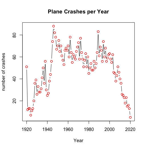
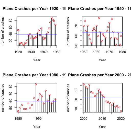
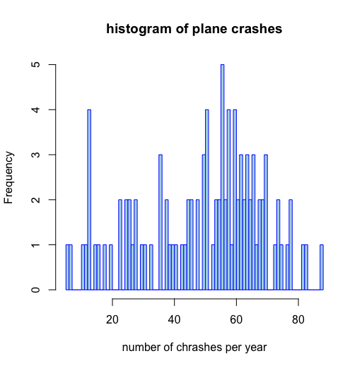
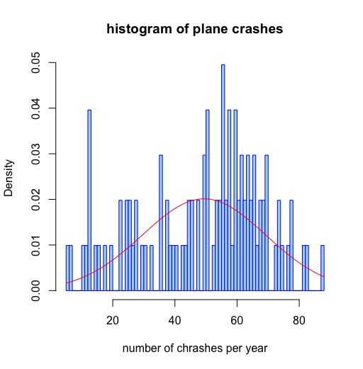
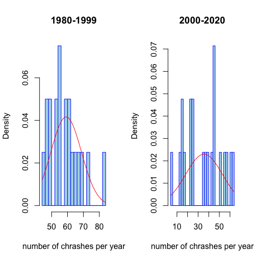
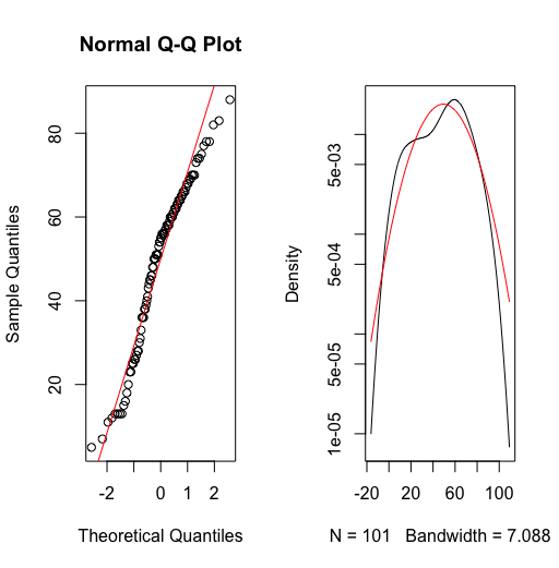
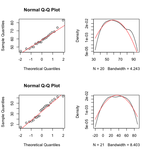
Plane crash data
|
1 2 3 4 5 6 7 8 9 10 11 12 13 14 15 16 17 18 19 20 21 22 23 24 25 26 27 28 29 30 31 32 33 34 35 36 37 38 39 40 41 42 43 44 45 46 47 48 49 50 51 52 53 54 55 56 57 58 59 60 61 62 63 64 65 66 67 68 69 70 71 72 73 74 75 76 77 78 79 80 81 82 83 84 85 86 87 88 89 90 91 92 93 94 95 96 97 98 99 100 101 102 103 104 105 106 107 108 109 110 111 112 113 114 115 116 117 118 119 120 121 122 123 124 125 126 127 128 129 130 131 132 133 134 135 136 137 138 139 140 141 142 143 144 145 146 147 148 149 150 151 152 153 154 155 156 157 158 159 160 161 162 163 164 165 166 167 168 169 170 171 172 173 174 175 176 177 178 179 180 181 182 183 184 185 186 187 188 189 190 191 192 193 194 195 196 197 198 199 200 201 202 203 204 205 206 207 208 209 210 211 212 213 214 215 216 217 218 219 220 221 222 223 224 225 226 227 228 229 230 231 232 233 234 235 236 237 238 239 240 241 242 243 244 245 246 247 248 249 250 251 252 253 254 255 256 257 258 259 260 261 262 263 264 265 266 267 268 269 270 271 272 273 274 275 276 277 278 279 280 281 282 283 284 285 286 287 288 289 290 291 292 293 294 295 296 297 298 299 300 301 302 303 304 305 306 307 308 309 310 311 312 313 314 315 316 317 318 319 320 321 322 323 324 325 326 327 328 329 330 331 332 333 334 335 336 337 338 339 340 341 342 343 344 345 346 347 348 349 350 351 352 353 354 355 356 357 358 359 360 361 362 363 364 365 366 367 368 369 370 371 372 373 374 375 376 377 378 379 380 381 382 383 384 385 386 387 388 389 390 391 392 393 394 395 396 397 398 399 400 |
# - - - - - - - - - - - - - - - - - - - - - - - - - - - - - - - - - - - - - - - # # A Simple Skript for planecrash data from: # http://www.planecrashinfo.com/database.htm # The aviation accident database includes: # All civil and commercial aviation accidents of scheduled and non-scheduled # passenger airliners worldwide, which resulted in a fatality # (including all U.S. Part 121 and Part 135 fatal accidents) # All cargo, positioning, ferry and test flight fatal accidents. # All military transport accidents with 10 or more fatalities. # All commercial and military helicopter accidents with greater than # 10 fatalities. # All civil and military airship accidents involving fatalities. # Aviation accidents involving the death of famous people. # Aviation accidents or incidents of noteworthy interest. # Database Format # Date: Date of accident, in the format - January 01, 2001 # Time: Local time, in 24 hr. format unless otherwise specified # Airline/Op: Airline or operator of the aircraft # Flight #: Flight number assigned by the aircraft operator # Route: Complete or partial route flown prior to the accident # AC Type: Aircraft type # Reg: ICAO registration of the aircraft # cn / ln: Construction or serial number / Line or fuselage number # Aboard: Total aboard (passengers / crew) # Fatalities: Total fatalities aboard (passengers / crew) # Ground: Total killed on the ground # Summary: Brief description of the accident and cause if known # to be done: histograms, t test?, types of chrashes, # country filter?, region filter, plane filter # text analysis, # - - - - - - - - - - - - - - - - - - - - - - - - - - - - - - - - - - - - - - - # # packages library("XML") library("quantmod") # - - - - - - - - - - - - - - - - - - - - - - - - - - - - - - - - - - - - - - - # # rm(list = ls(all = TRUE)) getwd() #system("ls") setwd("~/ownCloud/STA_Statistics/PlaneCrashData") # - - - - - - - - - - - - - - - - - - - - - - - - - - - - - - - - - - - - - - - # # get the available years url <- "http://www.planecrashinfo.com/database.htm" tables <- readHTMLTable(url,header=FALSE) years <- NULL for(i in 1:length(tables[[2]][,1])){ for(e in 2:length(tables[[2]][1,])){ years<-c(years,levels(tables[[2]][i,e])[i]) } } years years<-na.omit(as.numeric(years)) years # - - - - - - - - - - - - - - - - - - - - - - - - - - - - - - - - - - - - - - - # # get all data tables table.crash.all <- list() for(i in 1:length(years)){ url2 <- paste("http://www.planecrashinfo.com/", years[i],"/",years[i],".htm",sep="") assign(paste("table.crash.",years[i],sep=""),readHTMLTable(url2)) table.crash.all[[i]] <- get(paste("table.crash.",years[i],sep="")) print(paste("Year",years[i],"downloaded")) } #table.crash.all length(table.crash.all) save(table.crash.all,file="planecrashdata_list.RData") for(i in 1:length(years)){ data<-table.crash.all[[i]] save(data,file=paste("planecrashdata_",years[i],".RData",sep="")) } for(i in 1:length(years)){ data<-table.crash.all[[i]] write.csv(data,file=paste("planecrashdata_",years[i],".csv",sep="")) } # - - - - - - - - - - - - - - - - - - - - - - - - - - - - - - - - - - - - - - - # # Plane Crashes per Year years.crashes <- data.frame() for(i in 1:length(years)){ years.crashes[i,1] <- years[i] years.crashes[i,2] <- length(as.data.frame(table.crash.all[[i]])[,1]) } years.crashes rownames(years.crashes)<-years.crashes[,1] par(mfrow=c(1,1)) plot(years.crashes,type="b",main="Plane Crashes per Year", xlab="Year",ylab="number of crashes") points(years.crashes,col="red") par(mfrow=c(1,1)) setwd("/Users/impac/ownCloud/STA_Statistics/PlaneCrashData/plots") jpeg(file="Plane Crashes per Year-points.jpeg", width = 1080, height = 1080, pointsize = 12, quality = 75) plot(years.crashes,type="b",main="Plane Crashes per Year", xlab="Year",ylab="number of crashes") points(years.crashes,col="red") dev.off() jpeg(file="Plane Crashes per Year-bars.jpeg", width = 1080, height = 1080, pointsize = 12, quality = 75) plot(years.crashes,type="h",main="Plane Crashes per Year", xlab="Year",ylab="number of crashes") points(years.crashes,col="red") dev.off() jpeg(file="Plane Crashes per Year-steps.jpeg", width = 1080, height = 1080, pointsize = 12, quality = 75) plot(years.crashes,type="s",main="Plane Crashes per Year", xlab="Year",ylab="number of crashes") points(years.crashes,col="red") dev.off() par(mfrow=c(2,2)) plot(years.crashes[1:30,],type="h",main=paste("Plane Crashes per Year", years.crashes[1,1],"-",years.crashes[30,1]),xlab="Year", ylab="number of crashes") points(years.crashes[1:30,],col="red") abline(h=mean(years.crashes[1:30,2]),col="blue") plot(years.crashes[31:60,],type="h",main=paste("Plane Crashes per Year",years.crashes[31,1],"-",years.crashes[60,1]),xlab="Year",ylab="number of crashes") points(years.crashes[31:60,],col="red") abline(h=mean(years.crashes[31:60,2]),col="blue") plot(years.crashes[61:80,],type="h",main=paste("Plane Crashes per Year",years.crashes[61,1],"-",years.crashes[80,1]),xlab="Year",ylab="number of crashes") points(years.crashes[61:80,],col="red") abline(h=mean(years.crashes[61:80,2]),col="blue") plot(years.crashes[81:length(years.crashes[,1]),],type="h",main=paste("Plane Crashes per Year",years.crashes[81,1],"-",years.crashes[length(years.crashes[,1]),1]),xlab="Year",ylab="number of crashes") points(years.crashes[81:length(years.crashes[,1]),],col="red") abline(h=mean(years.crashes[81:length(years.crashes[,1]),2]),col="blue") #jpeg(file="Plane Crashes per Year.jpeg", width = 1080, height = 1080, pointsize = 12, quality = 75) #par(mfrow=c(2,2)) #plot(years.crashes[1:30,],type="h",main=paste("Plane Crashes per Year",years.crashes[1,1],"-",years.crashes[30,1]),xlab="Year",ylab="number of crashes") #points(years.crashes[1:30,],col="red") #abline(h=mean(years.crashes[1:30,2]),col="blue") #plot(years.crashes[31:60,],type="h",main=paste("Plane Crashes per Year",years.crashes[31,1],"-",years.crashes[60,1]),xlab="Year",ylab="number of crashes") #points(years.crashes[31:60,],col="red") #abline(h=mean(years.crashes[31:60,2]),col="blue") #plot(years.crashes[61:80,],type="h",main=paste("Plane Crashes per Year",years.crashes[61,1],"-",years.crashes[80,1]),xlab="Year",ylab="number of crashes") #points(years.crashes[61:80,],col="red") #abline(h=mean(years.crashes[61:80,2]),col="blue") #plot(years.crashes[81:length(years.crashes[,1]),],type="h",main=paste("Plane Crashes per Year",years.crashes[81,1],"-",years.crashes[length(years.crashes[,1]),1]),xlab="Year",ylab="number of crashes") #points(years.crashes[81:length(years.crashes[,1]),],col="red") #abline(h=mean(years.crashes[81:length(years.crashes[,1]),2]),col="blue") #dev.off() # - - - - - - - - - - - - - - - - - - - - - - - - - - - - - - - - - - - - - - - # # Histograms of the number of crashes par(mfrow=c(1,1)) hist(years.crashes[,2], nclass=length(years.crashes[,2]), freq=TRUE, main='histogram of plane crashes', xlab="number of chrashes per year", col = "lightblue", border = "blue") hist(years.crashes[,2], nclass=length(years.crashes[,2]), freq=FALSE, main='histogram of plane crashes',xlab="number of chrashes per year", col = "lightblue", border = "blue") curve(dnorm(x, mean=mean(years.crashes[,2]),sd=sd(years.crashes[,2])), add=TRUE, col="red") par(mfrow=c(1,2)) qqnorm(years.crashes[,2]) qqline(years.crashes[,2], col = 2) plot(density(years.crashes[,2]),log='y', main='') curve(dnorm(x, mean=mean(years.crashes[,2]), sd=sd(years.crashes[,2])), log="y", add=TRUE, col="red") # different periods par(mfrow=c(1,2)) # 1980-1999 #hist(years.crashes[61:80,2], nclass=20, freq=TRUE, # main='',xlab="number of chrashes per year", col = "lightblue", # border = "blue") hist(years.crashes[61:80,2], nclass=20, freq=FALSE, main='1980-1999',xlab="number of chrashes per year", col = "lightblue", border = "blue") curve(dnorm(x, mean=mean(years.crashes[61:80,2]),sd=sd(years.crashes[61:80,2])), add=TRUE, col="red") # 2000-2020 #hist(years.crashes[81:length(years.crashes[,1]),2], nclass=length(years.crashes[81:length(years.crashes[,1]),2]), freq=TRUE, main='',xlab="number of chrashes per year", col = "lightblue", border = "blue") hist(years.crashes[81:length(years.crashes[,1]),2], nclass=length(years.crashes[81:length(years.crashes[,1]),2]), freq=FALSE, main='2000-2020',xlab="number of chrashes per year", col = "lightblue", border = "blue") curve(dnorm(x,mean=mean(years.crashes[81:length(years.crashes[,1]),2]),sd=sd(years.crashes[81:length(years.crashes[,1]),2])), add=TRUE, col="red") par(mfrow=c(2,2)) qqnorm(years.crashes[61:80,2]) qqline(years.crashes[61:80,2], col = 2) plot(density(years.crashes[61:80,2]),log='y', main='') curve(dnorm(x, mean=mean(years.crashes[61:80,2]),sd=sd(years.crashes[61:80,2])), log="y", add=TRUE, col="red") qqnorm(years.crashes[81:length(years.crashes[,1]),2]) qqline(years.crashes[81:length(years.crashes[,1]),2], col = 2) plot(density(years.crashes[81:length(years.crashes[,1]),2]),log='y', main='') curve(dnorm(x, mean=mean(years.crashes[81:length(years.crashes[,1]),2]),sd=sd(years.crashes[81:length(years.crashes[,1]),2])), log="y", add=TRUE, col="red") # - - - - - - - - - - - - - - - - - - - - - - - - - - - - - - - - - - - - - - - # # boxplots par(mfrow=c(1,1)) boxplot(years.crashes[,2], main="number of plain crashes per year 1920 - 2020", xlab="", ylab="plain crashes per year") boxplot(years.crashes[,2], notch=TRUE, col=(c("gold","darkgreen")), main="number of plain crashes per year 1920 - 2020", ylab="plain crashes per year") years.crashes[1:30,3]<-rep("1920-1949",30) years.crashes[31:60,3]<-rep("1950-1979",30)278750 years.crashes[61:80,3]<-rep("1980-1999",20) years.crashes[81:length(years.crashes[,1]),3]<-rep("2000-2020",21) colnames(years.crashes)<-c("year","ncrashes","cat") boxplot(ncrashes~cat, data=years.crashes, notch=TRUE, col=(c("green","blue","blue","green")), main="number of plain crashes per year - groups", xlab="") # start from here # - - - - - - - - - - - - - - - - - - - - - - - - - - - - - - - - - - - - - - - # # - - - - - - - - - - - - - - - - - - - - - - - - - - - - - - - - - - - - - - - # # t test # independent 2-group t-test t.test(y~x) # where y is numeric and x is a binary factor # independent 2-group t-test t.test(y1,y2) # where y1 and y2 are numeric # paired t-test t.test(y1,y2,paired=TRUE) # where y1 & y2 are numeric # one sample t-test t.test(y,mu=3) # Ho: mu=3 t.test(years.crashes[61:80,2],years.crashes[81:length(years.crashes[,1]),2]) # Welch Two Sample t-test # # data: years.crashes[61:80, 2] and years.crashes[81:length(years.crashes[, 1]), 2] # t = 5.4142, df = 31.453, p-value = 6.268e-06 # alternative hypothesis: true difference in means is not equal to 0 # 95 percent confidence interval: # 14.70178 32.45536 # sample estimates: # mean of x mean of y # 59.15000 35.57143 # - - - - - - - - - - - - - - - - - - - - - - - - - - - - - - - - - - - - - - - # # rate of difference par(mfrow=c(3,1)) rate<-na.omit(ROC(years.crashes[,2])) plot(rate,type="l") plot(cumsum(rate),type="l") hist(rate, nclass=20) rate<-na.omit(ROC(years.crashes[61:80,2])) plot(rate,type="l") plot(cumsum(rate),type="l") hist(rate, nclass=20) rate<-na.omit(ROC(years.crashes[81:length(years.crashes[,1]),2])) plot(rate,type="l") plot(cumsum(rate),type="l") hist(rate, nclass=20) # - - - - - - - - - - - - - - - - - - - - - - - - - - - - - - - - - - - - - - - # # One big Table table.crash.one.table <- data.frame(table.crash.all[[1]],stringsAsFactors = TRUE) colnames(table.crash.one.table)<-c("date","location","type","fatalities") for(i in 2:length(years)){ data <- data.frame(table.crash.all[[i]],stringsAsFactors = TRUE) colnames(data)<-c("date","location","type","fatalities") table.crash.one.table <- rbind(table.crash.one.table,data) } table.crash.one.table # - - - - - - - - - - - - - - - - - - - - - - - - - - - - - - - - - - - - - - - # # create a time series object date <- gsub("Jan","01",table.crash.one.table[,1]) date <- gsub("Feb","02",date) date <- gsub("Mar","03",date) date <- gsub("Apr","04",date) date <- gsub("May","05",date) date <- gsub("Jun","06",date) date <- gsub("Jul","07",date) date <- gsub("Aug","08",date) date <- gsub("Sep","09",date) date <- gsub("Oct","10",date) date <- gsub("Nov","11",date) date <- gsub("Dec","12",date) gsub("/","-",table.crash.one.table[,4]) fatalities <- strsplit(gsub("/","-",table.crash.one.table[,4]),'-') number<-NULL for(i in 1:length(fatalities)){number<-c(number,fatalities[[i]][1])} #as.numeric(number) table.crash.one.table[,5]<-as.numeric(number) #strsplit(gsub("(","-",fatalities[[i]][2], fixed = TRUE),"-")[1] number2<-NULL for(i in 1:length(fatalities)){number2<-c(number2, strsplit(gsub("(","-",fatalities[[i]][2], fixed = TRUE),"-")[[1]][1])} number2 table.crash.one.table[,6]<-as.numeric(number2) colnames(table.crash.one.table)<-c("date","location","type", "fatalities","fatalities-passengers","fatalities-crew") #table.crash.one.table.xts <- xts(table.crash.one.table[,2:6], order.by=as.Date(date,"%d %m %Y")) #colnames(table.crash.one.table.xts)<-c("location","type","fatalities", #"passengerfatalities","crewfatalities") table.crash.one.table.xts <- xts(table.crash.one.table[,5:6], order.by=as.Date(date,"%d %m %Y")) colnames(table.crash.one.table.xts)<-c("totalfatalities","totalaboard") table.crash.one.table.xts$totalfatalities table.crash.one.table.xts$totalaboard plot(table.crash.one.table.xts$totalfatalities, main="Plane Crash Total Fatalities") plot(table.crash.one.table.xts$totalaboard, main="Plane Crash Total Aboard") plot(table.crash.one.table.xts$totalaboard, main="Plane Crash Total Aboard vs Total Fatalities") lines(table.crash.one.table.xts$totalfatalities,col="red") plot(table.crash.one.table.xts$totalaboard["2000/2020"], main="Plane Crash Total Aboard vs Total Fatalities",type="c") plot(table.crash.one.table.xts$totalaboard["2000/2020"], main="Plane Crash Total Aboard vs Total Fatalities",type="o") plot(table.crash.one.table.xts$totalaboard["2000/2020"], main="Plane Crash Total Aboard vs Total Fatalities",type="h") plot(table.crash.one.table.xts$totalaboard["2000/2020"], main="Plane Crash Total Aboard vs Total Fatalities",type="b") points(table.crash.one.table.xts$totalfatalities["2000/2020"],col="red") # - - - - - - - - - - - - - - - - - - - - - - - - - - - - - - - - - - - - - - - # # Total killed on the ground number3<-NULL for(i in 1:length(fatalities)){ sub <- gsub("(","-",fatalities[[i]][2], fixed = TRUE) sub <- gsub(")","-",sub, fixed = TRUE) number3<-c(number3,strsplit(sub,"-")[[1]][2]) } number3 table.crash.one.table[,7]<-as.numeric(number3) colnames(table.crash.one.table)<-c("date","location","type", "fatalities","fatalities-passengers","fatalities-crew","totalkilledontheground") table.crash.one.table.xts <- xts(table.crash.one.table[,5:7], order.by=as.Date(date,"%d %m %Y")) colnames(table.crash.one.table.xts)<-c("totalfatalities","totalaboard","totalkilledontheground") plot(table.crash.one.table.xts$totalkilledontheground, main="Plane Crash Total killed on the ground") plot(table.crash.one.table.xts$totalkilledontheground, main="Plane Crash Total killed on the ground",type="b") plot(table.crash.one.table.xts$totalkilledontheground, main="Plane Crash Total killed on the ground",type="c") # Martin Stoppacher # # office@martinstoppacher.com # # - - - - - - - - - - - - - - - - - - - - - - - - - - - - - - - - - - - - - - - # ################################################################################# |
My Sounds (Freesound.org)
This is a collection of my sounds at freesound.org. I try to keep the list up to date but sometimes there are more sounds available on freesound therefore please check out my freesound account and freesound in general. “Freesound is a collaborative database of Creative Commons Licensed sounds. Browse, download and share sounds.” – freesound.org
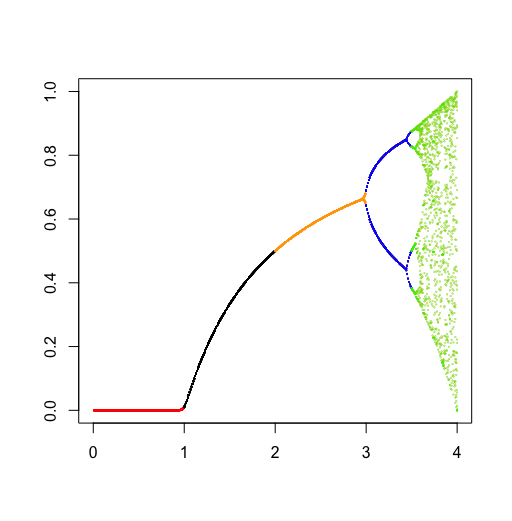
bifurcation tree with R
Lately i was exploring the logistic map function because i was fascinated again how chaotic behavior can arise from very simple circumstances (i.e. a rather simple equation).
Of course, i learned about this in school but never got a chance to write some code.
So here it is. 🙂
And here is some of the code i wrote:
|
1 2 3 4 5 6 7 8 9 10 11 12 13 14 15 |
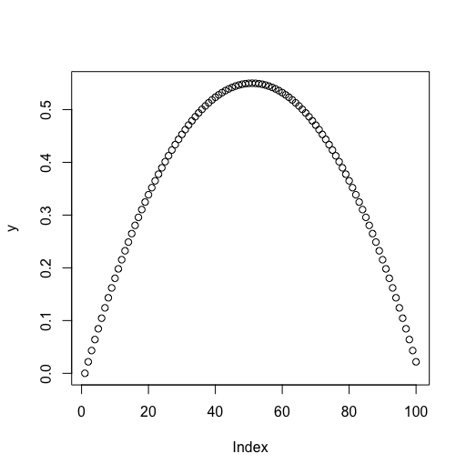
# - - - - - - - - - - - - - - - - - - - - - - - - - - - - - - - - - - - - - - - # # bifurcation tree, Logistic map # xn1=rxn(1-xn) rm(list = ls(all = TRUE)) r <- 2.2 # rate x <- 0.5 # population (r*x*(1-x)) r <- 2.2 (x <- seq(100,1)/100) y = r*x*(1-x) plot(y) |
|
1 2 3 4 5 6 7 8 9 10 11 12 13 |
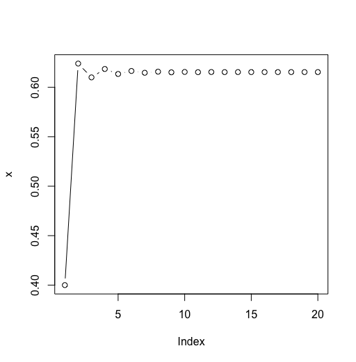
# - - - - - - - - - - - - - - - - - - - - - - - - - - - - - - - - - - - - - - - # # if the starting population is 0.1 r <- 2.6 x <- 0.1 for(i in 2:20){ (x[i] <- r*x[i-1]*(1-x[i-1])) print(i) print(x[i]) #Sys.sleep(0.5) } x plot(x, type="b") |
|
1 2 3 4 5 6 7 8 9 10 11 12 13 |
# - - - - - - - - - - - - - - - - - - - - - - - - - - - - - - - - - - - - - - - # # if the starting population is 0.8 r <- 2.6 x <- 0.8 for(i in 2:20){ (x[i] <- r*x[i-1]*(1-x[i-1])) print(i) print(x[i]) #Sys.sleep(0.5) } x plot(x, type="b") |

|
1 2 3 4 5 6 7 8 9 10 11 12 13 14 15 16 17 |
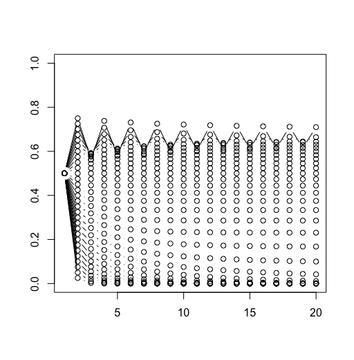
# - - - - - - - - - - - - - - - - - - - - - - - - - - - - - - - - - - - - - - - # # if we make variations to the initial population all of them stabilize plot(1:20,(1:20)/20,ylab="",xlab="",cex=0) for(e in ((1:9)/10)){ r <- 2.6 x <- e for(i in 2:20){ (x[i] <- r*x[i-1]*(1-x[i-1])) print(i) print(x[i]) #Sys.sleep(0.5) } x lines(x, type="b") } |

|
1 2 3 4 5 6 7 8 9 10 11 12 13 14 15 16 17 |
# - - - - - - - - - - - - - - - - - - - - - - - - - - - - - - - - - - - - - - - # # what does this look like if there are variations to the groth rate? plot(0,0, ylab="", xlab="", cex=0, xlim=c(1,20), ylim=c(0,1)) for(e in (1:30)/10){ r <- e x <- 0.5 for(i in 2:20){ (x[i] <- r*x[i-1]*(1-x[i-1])) print(i) print(x[i]) #Sys.sleep(0.5) } x lines(x, type="b") } |
|
1 2 3 4 5 6 7 8 9 10 11 12 13 14 15 16 17 18 19 |
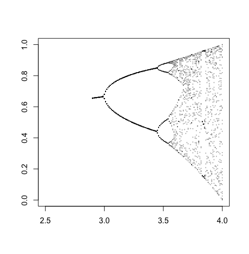
# - - - - - - - - - - - - - - - - - - - - - - - - - - - - - - - - - - - - - - - # # ploting more values but only the last plot(0,0, ylab="", xlab="", cex=0, xlim=c(2.5,4), ylim=c(0,1)) n<-300 m<-30 for(e in ((290:400)/100)){ print(r) r <- e x <- 0.1 for(i in 2:n){ (x[i] <- r*x[i-1]*(1-x[i-1])) print(r) print(x[i]) } x points(rep(r,(m+1)),x[(n-m):n], type="p", cex=0.2, lwd=0.2) } |
|
1 2 3 4 5 6 7 8 9 10 11 12 13 14 15 16 17 18 19 20 21 22 23 |
# - - - - - - - - - - - - - - - - - - - - - - - - - - - - - - - - - - - - - - - # # adding color plot(0,0, ylab="", xlab="", cex=0, xlim=c(0,4), ylim=c(0,1)) n<-100 m<-30 for(e in ((1:400)/100)){ print(r) r <- e x <- 0.6 for(i in 2:n){ (x[i] <- r*x[i-1]*(1-x[i-1])) print(r) print(x[i]) } x if(r<1)points(rep(r,(m+1)),x[(n-m):n], type="p", cex=0.2, lwd=0.2, col="red") if(r>=1&r<2)points(rep(r,(m+1)),x[(n-m):n], type="p", cex=0.2, lwd=0.2, col="black") if(r>=2&r<5)points(rep(r,(m+1)),x[(n-m):n], type="p", cex=0.2, lwd=0.2, col="orange") if(r>=3&r<=3.5)points(rep(r,(m+1)),x[(n-m):n], type="p", cex=0.2, lwd=0.2, col="blue") if(r>=3.5&r<=4)points(rep(r,(m+1)),x[(n-m):n], type="p", cex=0.2, lwd=0.2, col="green") } |
|
1 2 3 4 5 6 7 8 9 |
# - - - - - - - - - - - - - - - - - - - - - - - - - - - - - - - - - - - - - - - # # bifurcation tree as a function log.tree <- function(r=2, x=0.4, n=200){ for(i in 2:(n+1)){ (x[i] <- r*x[i-1]*(1-x[i-1])) } x <- x[2:(n+1)] } |
|
1 2 3 4 5 6 7 8 9 10 11 12 13 14 15 |
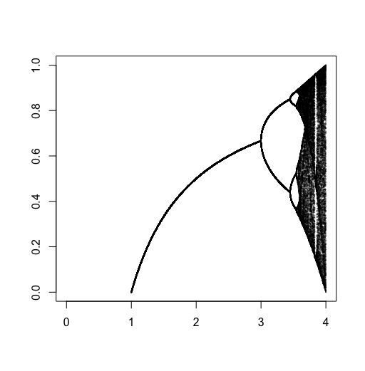
# - - - - - - - - - - - - - - - - - - - - - - - - - - - - - - - - - - - - - - - # # using the function with sapply point.count <- 50 # sets how many of the last observations to use r.seq <- seq(1,4,by=0.001) # a sequence for different rates plot(0,0, ylab="", xlab="", cex=0, xlim=c(0,4), ylim=c(0,1)) log.tree.points <- tail(sapply(r.seq, log.tree, x=0.1, n=3000),point.count) for(i in 1:length(r.seq)) points(rep(r.seq[i],point.count),log.tree.points[,i], cex=0.2, lwd=0.2) # - - - - - - - - - - - - - - - - - - - - - - - - - - - - - - - - - - - - - - - # # system.time(log.tree.points <- tail(sapply(r.seq, log.tree, x=0.1, n=300),point.count)) system.time(log.tree.points <- tail(sapply(r.seq, log.tree, x=0.1, n=3000),point.count)) system.time(log.tree.points <- tail(sapply(r.seq, log.tree, x=0.1, n=30000),point.count)) |
|
1 2 3 4 |
# Martin Stoppacher # # office@martinstoppacher.com # # - - - - - - - - - - - - - - - - - - - - - - - - - - - - - - - - - - - - - - - # ################################################################################# |
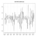
Creating sounds out of financial data.
|
1 2 3 4 5 6 7 8 9 10 11 12 13 14 15 16 17 18 19 20 21 22 23 24 25 26 27 28 29 30 31 32 33 34 35 36 37 38 39 40 41 42 43 44 45 46 47 48 49 50 51 52 53 54 55 56 57 58 59 60 61 62 63 64 65 66 67 68 69 70 71 72 73 74 75 76 77 78 79 80 81 82 83 84 85 86 87 88 89 90 91 92 93 94 95 96 97 98 99 100 101 102 103 104 105 106 107 108 109 110 111 112 113 114 115 116 117 118 119 120 121 122 123 124 125 126 127 128 129 130 131 132 133 134 135 136 137 138 139 140 141 142 143 144 145 146 147 148 149 150 151 152 153 154 155 156 157 158 159 160 161 162 163 164 165 166 167 168 169 170 171 172 173 174 175 176 177 |
# - - - - - - - - - - - - - - - - - - - - - - - - - - - - - - - - - - - - - - - - - - - # # install.packages("seewave") require("seewave") install.packages("tuneR") require("tuneR") #rm(list = ls(all = TRUE)) # clear current workspace # setwd("/Users/martinstoppacher/R Analysis/3_Index Sounds/") library("quantmod") getSymbols("^GSPC",from=1900) head(GSPC) tail(GSPC) jpeg(filename = "SP500.jpg1975-2015.jpg", width=880,height=880,res=100) plot(Cl(GSPC),main="S&P 500 Index (closing prices)") dev.off() summary(Cl(GSPC)) jpeg(filename = "SP500.jpg1975-1985.jpg", width=880,height=880,res=100) plot(Cl(GSPC)["1975/1985"],main="S&P 500 Index 1975-1985 (closing prices)") dev.off() jpeg(filename = "SP500.jpg1985-1995.jpg", width=880,height=880,res=100) plot(Cl(GSPC)["1985/1995"],main="S&P 500 Index 1985-1995 (closing prices)") dev.off() jpeg(filename = "SP500.jpg1995-2005.jpg", width=880,height=880,res=100) plot(Cl(GSPC)["1995/2005"],main="S&P 500 Index 1995-2005 (closing prices)") dev.off() jpeg(filename = "SP500.jpg2005-2015.jpg", width=880,height=880,res=100) plot(Cl(GSPC)["2005/2015"],main="S&P 500 Index 2005-2015 (closing prices)") dev.off() jpeg(filename = "SP500.jpg 1975-2005 4decades-new.jpg", width=880,height=880,res=100) plot(as.numeric(Cl(GSPC)["1975/1984"]),main="S&P 500 Index 1975-1985 - 4 decades (closing prices)",ylim=c(0,2100),type="l",ylab="index values",xlab="days (10 year)") lines(as.numeric(Cl(GSPC)["1985/1994"]),col="red") lines(as.numeric(Cl(GSPC)["1995/2004"]),col="blue") lines(as.numeric(Cl(GSPC)["2005/2015"]),col="green") legend("topleft", legend = c("1975-1984","1985-1994","1995-2004","2005-2014") , lty = 1, col = c("black","red","blue","green")) dev.off() jpeg(filename = "SP500.jpg 1975-2005 4decades percent-new2.jpg", width=880,height=880,res=100) plot((as.numeric(Cl(GSPC)["1975/1984"])/as.numeric(Cl(GSPC)["1975/1984"][1])-1),main="S&P 500 Index 1975-1985 - 4 decades (percent changes)",ylim=c(-0.4,2.3),type="l",ylab="index values",xlab="days (10 year)") lines((as.numeric(Cl(GSPC)["1985/1994"])/as.numeric(Cl(GSPC)["1985/1994"][1])-1),col="red") lines((as.numeric(Cl(GSPC)["1995/2004"])/as.numeric(Cl(GSPC)["1995/2004"][1])-1),col="blue") lines((as.numeric(Cl(GSPC)["2005/2014"])/as.numeric(Cl(GSPC)["2005/2014"][1])-1),col="green") legend("topleft", legend = c("1975-1984","1985-1994","1995-2004","2005-2014") , lty = 1, col = c("black","red","blue","green")) dev.off() jpeg(filename = "SP500.jpg 1975-2005 4otherdecades percent2-new.jpg", width=880,height=880,res=100) plot(as.numeric(Cl(GSPC)["1980/1989"])/as.numeric(Cl(GSPC)["1980/1989"][1]),main="S&P 500 Index 1975-2015 - new truncation - (percent changes)",ylim=c(0.6,4.2),type="l",ylab="index values",xlab="days (10 year)",col="yellow") lines(as.numeric(Cl(GSPC)["1975/1979"])/as.numeric(Cl(GSPC)["1975/1979"][1]),col="red") lines(as.numeric(Cl(GSPC)["1990/1999"])/as.numeric(Cl(GSPC)["1990/1999"][1]),col="black") lines(as.numeric(Cl(GSPC)["2000/2009"])/as.numeric(Cl(GSPC)["2000/2009"][1]),col="blue") lines(as.numeric(Cl(GSPC)["2010/2014"])/as.numeric(Cl(GSPC)["2010/2014"][1]),col="green") legend("topleft", legend = c("1975-1979","1980-1989","1990-1999","2000-2009","2010-2014") , lty = 1, col = c("red","yellow","black","blue","green")) dev.off() library("PerformanceAnalytics") Cl(GSPC)["2010/2015"]/as.numeric(Cl(GSPC)["2005/2015"][1]) charts.PerformanceSummary(,main="",xlab="") # percent jpeg(filename = "SP500.jpg1975-1985-percent.jpg", width=880,height=880,res=100) plot(Cl(GSPC)["1975/1985"]/as.numeric(Cl(GSPC)["1975/1985"][1]),main="S&P 500 Index 1975-1985 (closing prices)") dev.off() jpeg(filename = "SP500.jpg1985-1995-percent.jpg", width=880,height=880,res=100) plot(Cl(GSPC)["1985/1995"]/as.numeric(Cl(GSPC)["1985/1995"][1]),main="S&P 500 Index 1985-1995 (closing prices)") dev.off() jpeg(filename = "SP500.jpg1995-2005-percent.jpg", width=880,height=880,res=100) plot(Cl(GSPC)["1995/2005"]/as.numeric(Cl(GSPC)["1995/2005"][1]),main="S&P 500 Index 1995-2005 (closing prices)") dev.off() jpeg(filename = "SP500.jpg2005-2015-percent.jpg", width=880,height=880,res=100) plot(Cl(GSPC)["2005/2015"]/as.numeric(Cl(GSPC)["2005/2015"][1]),main="S&P 500 Index 2005-2015 (closing prices)") dev.off() GSPC.cl.close <- diff(Cl(GSPC)) tail(GSPC.cl.close,20) jpeg(filename = "SP500-first-difference-example.jpg", width=880,height=880,res=100) plot(tail(GSPC.cl.close,200),main="S&P 500 first difference") dev.off() ## GSPC.cl.close.roc <- ROC(Cl(GSPC)) tail(GSPC.cl.close.roc,5) #prices <- Cl(GSPC) # ROC is log diff! #log_returns <- diff(log(prices), lag=1) #tail(log_returns) jpeg(filename = "SP500-first-roc-example.jpg", width=880,height=880,res=100) plot(tail(GSPC.cl.close.roc,200),main="S&P 500 first difference") dev.off() ## dax.roc <- na.omit(ROC(Cl(GSPC)))*100 plot(head(dax.roc,20)) plot(dax.roc) # standard if(abs(max(dax.roc))>abs(min(dax.roc))){ dax.roc.standard <- as.numeric(dax.roc/max(dax.roc)) }else{ dax.roc.standard <- as.numeric(dax.roc/abs(min(dax.roc))) } plot(dax.roc.standard,type="l") w<-dax.roc.standard f=41000 savewav(w,f=f ,filename = "xyz.wav") aw<-readWave("xyz.wav") play(aw) f=10000 savewav(w,f=f ,filename = "xyz.wav") aw<-readWave("xyz.wav") play(aw) f=5000 savewav(w,f=f ,filename = "xyz.wav") aw<-readWave("xyz.wav") play(aw) dax.roc <- as.numeric(dax.roc) dax.roc2 <- NULL for(i in 1:length(dax.roc)){ dax.roc2 <- rbind(dax.roc2,((dax.roc[i]+dax.roc[i+1])/2)) } lines <- NULL for(i in 1:length(dax.roc)){ line <- rbind(dax.roc[i],dax.roc2[i]) lines <- rbind(lines,line) } dax.roc <- na.omit(lines) tail(dax.roc) dax.roc <- na.omit(ROC(SMA(Cl(GSPC),n=500)))*100 dax.roc <- na.omit(ROC(Cl(GDAXI)))*100 dax.roc.standard <- as.numeric(dax.roc/max(dax.roc)) dax.roc.standard <- as.numeric(dax.roc/min(dax.roc)) hist(dax.roc.standard) w<-na.omit(SMA(dax.roc.standard,n=100)) w<-dax.roc.standard for(i in 1:5){ w<-c(w,w) } f=32000 savewav(w,f=f ,filename = "xyz.wav") aw<-readWave("xyz.wav") play(aw) # Martin Stoppacher # # office@martinstoppacher.com # # - - - - - - - - - - - - - - - - - - - - - - - - - - - - - - - - - - - - - - - # ################################################################################# |
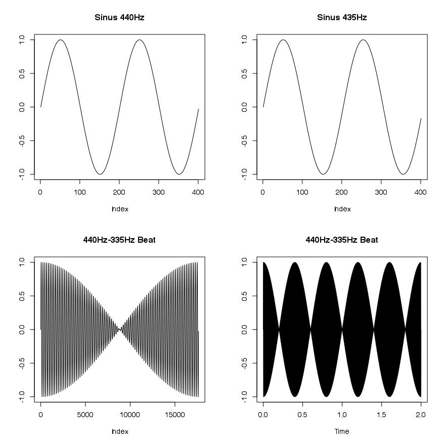
Creating a beat frequency interference with R
A beat frequency is a mix of two frequencies which are very close to each other but not similar. The trick is that they are to close to each other to be separated by the human ear as two distinct frequencies, thus generating a single tone with fluctuating amplitude behavior – a periodic change in volume. In Fact this effect just appears within the human brain, therefore the two tones can be measured physically by using the appropriate instruments. Further more the effect also works in a binaural situation where one ear can only hear one frequency respectively.
The following graphic shows two almost similar sinus waves, one at 440 Hz and one slightly below, at 435 Hz. The sound data is produced for exactly 2 seconds of time at a 44100 Hz sample rate, giving us 88200 sample points for 2 seconds. The first three demonstrations of the graph show only the beginning of the wave whereas the last one presents the combination of both signals for the complete 2 seconds.
Basically a combination of two sinus waves can be mathematically represented by:
![]() And if we assume that both amplitudes are the same we get the reduced form by:
And if we assume that both amplitudes are the same we get the reduced form by:
![]()
It is interesting to understand that the resulting frequency of the beat, i.e. the recognized periodic fluctuation of volume, is given by:
![]()
440Hz – Sinus – 2 seconds
435Hz – Sinus – 2 seconds
435 & 440Hz – Sinus – resulting beat frequency – 2 seconds
The oscillations in this post are simple created in R by using standard mathematical functions in combination with the time series package in R. In addition the seewave package is used to store the sinus waves as a .wav file to the system.
|
1 2 |
install.packages("seewave") require("seewave") |
The time series package handles data as equispaced points in time. This is in accordance with the sampling of continuous sound signals as the become digitized. A common used sampling frequency for CD quality is 44.1 kHz which results in 88.2k sample points for a length of 2 seconds.
|
1 2 3 4 5 6 7 8 9 10 11 12 13 14 15 |
s1<-sin(2*pi*440*seq(0,2,length.out=88200)) s1<-ts(data=s1, start=0, frequency=44100) jpeg(filename = "440Hz Sinus.jpg", width=880,height=880,res=100) plot(head(s1,401),type="l",ylab="") dev.off() s2<-sin(2*pi*435*seq(0,2,length.out=88200)) s2<-ts(data=s2, start=0, frequency=44100) jpeg(filename = "435Hz Sinus.jpg", width=880,height=880,res=100) plot(head(s2,401),type="l",ylab="") dev.off() s3<-(s1+s2)/2 |
For ease of use the summation of the amplitude 2a becomes reduced to a by division.
|
1 2 3 4 |
f<-44100 savewav(s1,f=f ,filename = "s1.wav") savewav(s2,f=f ,filename = "s2.wav") savewav(s3,f=f ,filename = "s3.wav") |
The graphical representation of the sound can easily be saved as a .jpg file to the system.
|
1 2 3 4 5 6 7 |
jpeg(filename = "435Hz-440Hz-beatsfrequency-4plots.jpg", width=880,height=880,res=100) par(mfrow=c(2,2)) plot(head(s1,401),type="l",ylab="",main="Sinus 440Hz") plot(head(s2,401),type="l",ylab="",main="Sinus 435Hz") plot(head(s3,17640),type="l",ylab="",main="440Hz-335Hz Beat") plot(s3,type="l",ylab="",main="440Hz-335Hz Beat") dev.off() |
In addition to the sample above we can also see and hear what it is like when the beat effect fades out and the brain starts to recognize two different tones. Therefore the next few examples present the resulting wave after summing two different frequencies, where one is always 440 Hz.
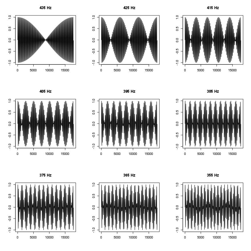
435 & 440Hz – Sinus – resulting beat frequency – 2 seconds
425 & 440Hz – Sinus – resulting (beat) frequency – 2 seconds
415 & 440Hz – Sinus – resulting (beat) frequency – 2 seconds
405 & 440Hz – Sinus – resulting (beat) frequency – 2 seconds
395 & 440Hz – Sinus – resulting (beat) frequency – 2 seconds
485 & 440Hz – Sinus – resulting (beat) frequency – 2 seconds
|
1 2 3 4 5 6 7 8 9 10 11 12 13 14 15 16 17 |
jpeg(filename = "beatsfrequency-9examples.jpg", width=880,height=880,res=100) par(mfrow=c(3,3)) for(i in 1:9){ e<-445-i*10 s1<-sin(2*pi*440*seq(0,2,length.out=88200)) s1<-ts(data=s1, start=0, frequency=44100) s2<-sin(2*pi*e*seq(0,2,length.out=88200)) s2<-ts(data=s2, start=0, frequency=44100) s3<-s1+s2 #jpeg(filename = "beatsfrequency.jpg", width=880,height=880,res=100) plot(head(s3/2,17640),type="l",ylab="",xlab="",main=paste(e,"Hz")) #plot(s3,type="l") #dev.off() f<-44100 savewav((s3/2),f=f ,filename = paste(e,"Hz - 440Hz-beat.wav")) } dev.off() |
- http://cran.r-project.org/web/views/TimeSeries.html
- http://cran.r-project.org/web/packages/seewave/index.html
Latex code for the Formulas above:
|
1 2 3 4 5 6 7 8 9 10 11 12 13 |
sin(2 \pi f_1t)+sin(2 \pi f_2t)=2sin(2 \pi \frac{f_1+f_2}{2} t)sin(2 \pi \frac{f_1-f_2}{2} t) x=(a_2-a_1)cos \omega_2t+2a_1cos\frac{\omega_1+\omega_2}{2}tcos\frac{\omega_2-\omega_1}{2}t x=2a_1cos\frac{\omega_1+\omega_2}{2}tcos\frac{\omega_2-\omega_1}{2}t \omega_a=\frac{\omega_1+\omega_2}{2} \omega_b=\frac{\omega_2-\omega_1}{2} \omega_s=\omega_2-\omega_1 f_s=f_2-f_1 |